Future Climate and Impacts

The Paleoclimate Record

Ice Core Measurements

Scientists have developed a technique by which global mean sea-surface temperatures can be deduced from measurements of the isotopic fractionation of oxygen in ice cores. This technique provides us with estimates of sea-level air temperatures over the past 160,000 years.

In order to establish the reliability of such measurements, paleoclimatologists have conducted a number of tests to calibrate this "paleoclimate thermometer" in the ice.

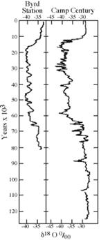
Figure 1. Ice-core oxygen isotopic measurements from Greenland (right hand side) and from Antarctica (left hand side). The isotope measurements can be interpreted to yield the global sea surface temperatures to ~160,000 years ago (colder temperatures to the left). The two traces are consistent with each other and depict the most recent glacial period, ending ~15,000 years ago.

Figure 1 shows an intercalibration of two sets of ice core isotopic measurements, one from Byrd Station in the Southern Hemisphere, and the other from Camp Century in the Northern Hemisphere. A decrease of one part per million (ppm) in the d¹⁸ O measurement is equivalent to a reduction in temperature of approximately 1.5^oC at the time that the water evaporated from the oceans.

Clearly the two sets of measurements are correlated, both showing the temperature reduction of the most recent Pleistocene glacial outbreak between 60,000 and 15,000 years ago. The warming trend to the present interglacial period started around 15,000 years ago. The dates for such measurements are obtained using models of ice deposition and flow.

Measurements of other isotopic ratios (such as light hydrogen to heavy hydrogen) in ice also provide important climate information.

The ice-core oxygen isotope measurements are complemented by studies of the composition of ancient air trapped in bubbles in the ice. The top panel of Figure 2 is a micro-photograph of an ice-core slice, clearly showing trapped bubbles. The ice is brought back to a laboratory and heated carefully in a vacuum chamber (to avoid contamination by modern air), releasing the ancient air for analysis.

The bottom panel of Figure 2 shows the results of ice bubble analysis for the atmospheric gas methane (CH4). The dots in the lower panel of Figure 2 represent ice measurements of methane, while the asterix represents atmospheric measurements of the methane abundance global average from the late 1970's. These analyses have shown that methane concentrations have hardly changed over most of the 160,000 year period, staying at values near 750 parts per billion. At about the time of the industrial revolution, however, methane concentrations rose, due in part to the production of the gas by enteric processes in cattle, anaerobic processes in rice paddies, and other human-driven activities. The recent rise in methane from pre-industrial levels is more than a factor of 2!

We have seen how ice cores can provide information on both temperatures and atmospheric composition for ancient times. Let's put the two pieces of evidence together and assemble a more detailed 160,000 year record of climate. Figure 3 shows the time series of ice-core data for temperature (oxygen isotope measurements) and for carbon dioxide and methane abundances (ice bubble measurements). The most recent rise in methane and carbon dioxide is not shown on this scale. The comparison is dramatic - all three curves show similar features!

The top panel of Figure 3 shows the temperature data for the past 180,000 years. The present (near left-hand side of graph) is relatively warm compared with the last period when glaciers covered Michigan ~18,000 years ago. The period of extensive cooling was marked by repeated advances and retreats of the glaciers.

Both methane and carbon dioxide correlate with temperature - i.e., an increase in temperature is associated with an increase in the abundance of both these two gases. It is unclear whether the gas abundance changes are a consequence of the temperature changes or vice versa.

Correlations such as these are difficult to interpret. It is hard to unravel the chain of cause and effect when a poorly understood feedback process is at play. Additional evidence for these processes are sought.. As we shall soon discuss, useful additional evidence comes from a study of changes in the Earth's orbit.

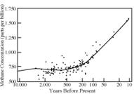
Figure 2. Ancient air found in bubbles trapped in ice cores (above, temporary picture) may be carefully analyzed to provide information on the atmospheric composition.

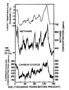
Figure 3. Correlations between the Ice Core measurements of paleoclimate temperatures and abundances of methane and carbon dioxide.

Deep Sea Sediment Analysis

Figure 4. A micro-photograph of small skeleton-bearing plankton sea creatures. When such creatures die, their shells fall to the bottom of the ocean, carrying the tell-tail oxygen isotopic ratio appropriate to the temperature of the surface waters where they lived.

The paleoclimate record discussed above goes back about 160,000 years. Compared with the history of the Earth, this is a very short period of time indeed. We can go back farther, however, using measurements made of oxygen isotope ration in deep sea cores, drilled from the ocean floor.

Analysis of oxygen isotopic ratios of ocean and atmospheric water oxygen isotopes has shown ocean surface sea water becomes enriched in heavy oxygen due to the temperature-dependent evaporation process. It follows that sea creatures living in these waters will possess shells containing more heavy oxygen. The proportion of heavy oxygen in sea shells (consisting of calcium carbonate -- CaCO₃) will go up in years when the temperature is colder and will go down in years when the temperature is warmer (exactly the opposite behavior to the heavy oxygen in glacial ice discussed above). This isotopic fractionation process was demonstrated in the laboratory by Harold Urey (the same Urey who was Stanley Miller's thesis advisor). In the 1950's, Urey performed a controlled laboratory experiment with plankton. He grew these tiny shelled creatures at different temperatures and was able to demonstrate the temperature dependence of the oxygen isotopic fractionation in the shells (i.e. the higher the temperature of the water, the smaller the ratio of heavy-to-light oxygen in the calcium carbonate of the shells).

Several deep sea cores have since been analyzed to determine the oxygen isotopic ratio of ancient calcium carbonate. It is from these these measurements and careful calibrations that we can obtain a record of sea surface temperatures that goes back almost 1 million years!

Figure 5. The Paleoclimate Temperature Record
at various time scales.

Figure 5 shows the million-year paleoclimate record, together with more detailed records of successively later times. To generate this figure, additional information has been used from the techniques noted on the right hand side of the diagram. It should be remembered that 1 million years represent only about one fiftieth of one percent of the Earth's lifetime.

We start our discussion with the one-million-year time series (Figure 5, Panel e). Note that the record from the deep sea sediments shows cycles of alternating cold and warm periods with a period of about 100,000 years. Superimposed on this long-term cycle are multiple excursions on shorter time scales. Clearly Michigan has been subject to many periods of glaciation over the past million years!

If we focus on the last 150,000 years only (Panel d), we see the glacial/interglacial features already indicated in Figure 3. The recent warming trend started in ~15,000 years ago (Panel c), when the glaciers last left Michigan. This warming coincides with the development of human civilization.

Panel c also shows a phenomenon of interest to us - the Younger Dryas. This was a short-lived period lasting about 700 years that occurred 10,000 years ago, when the general warming trend was interrupted by a sudden cooling. The term Younger Dryas was coined from the herbaceous plant "dryas" that covered much of the landscape during the colder time period. Evidence for this sudden cooling came from the study of ancient pollen grains found in sediments, which showed a abrupt change from pre and postglacial forests to glacial shrubs and then back again. This climate "jump" was also seen in ice core measurements of CO₂. The Younger Dryas provides dramatic evidence for rapid jumps in climate. We shall see in a later lecture, this phenomenon should be taken as a warning of possible things to come if rapid human-induced climate change continues.

Panel b of Figure 5 shows the record of the past 1,000 years. The climate about 1,000 years ago was relatively warm and dry (wine was grown in England!). We know from history that this was also the period that the Vikings ran out of room in Scandinavia and colonized Greenland (remember, it doesn't look very green now). Unfortunately for them, the period of relatively clement climate was replaced by colder conditions during the famous "Little Ice Age" and Greenland became uninhabitable again. The Little Ice Age is celebrated in paintings by Breugel of frozen rivers and streams in Holland. We are clearly seeing a connection between human activities and climate.

The most recent 200 years are shown in Panels a and b. During this time, global human activity signifigantly expanded and industrial revolution flourished. The graphs show that warming has continously increased (with a few interruptions), resulting that the 1980's has been the warmest decade of this of the century.

2. Causes of Paleoclimate Change

Figure 6. Ice Ages through Geologic Time

It is clear from the above discussion that climate change is constant - and that it occurs at all time scales. We next need to discuss the causes for paleoclimate change. In this discussion, we will start with the most ancient changes and move to the more recent changes. Of course, much of what follows is speculation and our picture will undoubtedly change as new paleo-climatological techniques are developed.

Although the basic causes of climate change are still not fully understood, many clues have been collected. Possible causes include:

Changes in solar output
Changes in Earth's orbit
Changes in the distribution of continents
Changes in the concentration of Greenhouse Gases in the atmosphere

We will separately consider climate changes over several different time scales: 1) the long term (100's million years); 2) medium term (1 million years); 3) short term (160,000 years) and 4) modern period (last few centuries).

Long-Term Changes

The long term (100's million years) paleoclimate record, shown in Figure 6, is characterized by relatively few, isolated glacial outbreaks - the great Ice Ages. We need to seek a factor, or a combination of factors, that could change the climate in this way over these long periods. The time scales and nature of the record argue against solar output and Earth's orbit changes to explain the great Ice Ages.

Radiation from the Sun is not constant, but varies at least by ~0.1 to 0.2%. There is a 22 year cycle of sunspots that causes a similar 22 year cycle of solar radiation. This cycle is thought by many scientists to play a minor role in climate change (though this is still subject to heated debate). Over longer periods, it is known that solar activity changes (as recorded by number of sunspots). It is interesting to note, for example, that during the "Maunder Minimum" (~1645-1715) few if any sunspots were seen. This corresponds to the peak time of the Little Ice Age.

Sunspot cycles have much too short a period to explain the great Ice Ages and we need to look for variations in solar output over much longer time intervals. Here we can appeal to plasma physics and to what is known about stellar evolution. Solar physicists believe that stars like the Sun brighten slowly over billions of years. In fact, the sun is thought to have been 30% dimmer 3 billion years ago than it is today. This slow increase in solar radiation with time does not help us explain the great Ice Ages, however, since one would then expect a record that followed the slow curve of solar radiation rather than the episodic plot of Figure 6. Although it is based on fundamental physical principles, the dim early sun is not an immediately helpful concept for paleoclimatologists. It is often called the "Faint Young Sun Paradox" since, if the sun were really that dim, one would have expected quite a different story for planetary evolution.

Changes in the nature of the Earth's orbit around the Sun, known as Milankovitch Cycles, occur over too short time scales to explain the long term climate change. These cycles are discussed below with reference to the medium-term changes.

So what then caused the Great Ice Ages? Let us consider the possibility of changes in the atmospheric greenhouse effect.

Our best guess today is associated with the very slow process known as "Plate Tectonics" and its influence on the atmospheric greenhouse effect. We will discuss Plate Tectonics in greater detail later on in this course. For the moment, it is sufficient to know that the continents (plates) "drift" on top of a fluid substrate over geologic time. When plates collide, some material can be pushed under the Earth's crust in a process known as "subduction", leading to increased volcanism.

Over the time scale of 300 million years (back to the last known Great Ice Age - the Gondwanan, see Figure 6), the continental plates have moved greatly. Figure 7a shows the distribution of continents today, together with the areas showing evidence of Gondwanan glaciation.

Figure 7. Top panel shows distribution of today's continents and regions of glaciation associated with the Gondwana Ice Age. Bottom panel shows the supercontinent Pangea (~300 million years ago), with the continents reassembled according to the theory of continental drift.

Figure 7b shows the locations of the continents ~300 million years ago when they were assembled into the great supercontinent Pangaea. It can be seen that the regions showing glaciation were all assembled near the South Pole.

The question remains as to why the temperatures dropped. Perhaps the answer lies in changes in the natural (non-biogenic) production rate of carbon dioxide - the number one greenhouse gas. We know that CO₂ is produced in volcanoes and in the mid-ocean trenches. It is lost by being slowly absorbed in the oceans. Both of these processes are very slow - about the right time scales to explain the great Ice Ages.

A drop in the production rate of carbon dioxide by volcanism would reduce the atmospheric greenhouse effect and lead to lower temperatures. We may speculate that the Gondawanan Ice Age started when the moving continental plates first assembled in Pangea (like bumper cars), they had to go through a readjustment period before drifting apart again. Perhaps, during the readjustment period, the production of carbon dioxide dropped, leading to the Gondwanan Ice Age.

Figure 8 shows how carbon dioxide is produced by volcanism and sea-floor spreading. During times of rapid spreading, increased volcanic activity, coupled with higher ocean levels and reduced chemical weathering of rocks, may promote global warming by enriching the CO₂ content of the atmosphere. Similarly, global cooling may result from stalled or slowed spreading.

Figure 8. The Earth is composed of a series of moving plates whose motion may influence climate change on long time scales.

Medium-Term Changes

The medium term changes in paleoclimate temperatures were illustrated by Figure 5e, above. This period, called the Pleistocene, was characterized by semi-regular advances and retreats of the glaciers during the most recent (and continuing) Great Ice Age.

The best clue for explaining these changes comes from a consideration of the Milankovitch cycles, changes in the orbital characteristics of the Earth.

Milankovitch Cycles

There are three types of orbital change of relevance to our discussion. These were first described by the Yugoslavian astronomer Milutin Milankovitch who first proposed the idea of a climate connection in the 1930's.

Figure 9. Eccentricity changes on a ~100,000 year cycle.

The basic premise of the theory is that, as the Earth travels through space, three separate cyclic movements combine to produce variations in the amount of solar energy falling on the Earth. Figure 9 illustrates the first type of orbital change, dealing with the changes in the shape of the Earth's orbit (eccentricity) as the Earth rotates about the Sun. The more eccentric the orbit the more elliptical the orbital shape.

It turns out that the Earth's orbit goes from quite elliptical to nearly circular in a cycle with a period of ~100,000 years. Presently, we are in a period of low eccentricity (~3%) and this gives us a seasonal change in solar energy of ~7%. When the eccentricity is at its peak (~9%), the "seasonality" reaches ~20%. In addition a more eccentric orbit will change the length of seasons in each hemisphere by changing the length of time between the vernal and automnal equinoxes.

The second Milankovitch cycle takes about 41,000 years to complete and involves changes in tilt (obliquity) of the Earth's axis (Figure 10). Presently the Earth's tilt is 23.5°, but the 41,000 year cycle varies from ~22° to 24.5°. The smaller the tilt, the less seasonal variation there is between summer and winter at middle and high latitudes.

For small tilt, the winters would tend to be milder and the summers cooler. This would lead to more glaciation.

The third cycle is due to precession of the spin axis (as in a spinning top) and occurs over a ~23,000 year cycle. Presently, the Earth is closest to the Sun in January and farther away in July. Due to precession, the reverse will be true in ~11,000 years. This will give the Northern Hemisphere more severe winters.

Figure 11 shows the correlation of the Milankovitch cycles with the paleoclimate records for the past million years. There is a good correlation, between periods of low eccentricity and glacial periods. A detailed view of the interglacial periods of the past ~160,000 years also shows evidence of the 41,000 year and 23,000 years cycles.

Other factors which work in conjunction with the Earth's orbital changes include:

The amount of dust in the atmosphere
The reflectivity of the ice sheets
The concentration of greenhouse gases
The changing characteristics of clouds
The rebounding of land, having been depressed by ice.

The Milankovitch cycles may help explain the advance and retreat of ice over periods of 10,000 to 100,000 years. They do not explain what caused the Ice Age in the first place.

When all the Milankovitch cycles (alone) are taken into account, the present trend should be towards a cooler climate in the Northern Hemisphere, with extensive glaciation.

Figure 10. (Temporary picture) Changes in tilt (obliquity) and precession occur on time scales of 41,000 years and ~23,000 years, respectively.

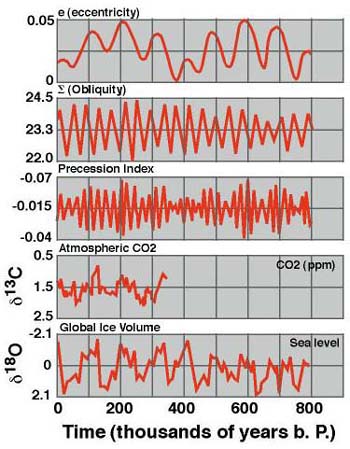
Figure 11. Correlation of the Milankovitch cycles and paleoclimate change.

Short-Term Changes

The glacial-interglacial variations observed over the 160,000 year record of Figure 6 are explained in part by solar forcing due to the Milankovitch theory. However, it remains to explain the observed correlation between the greenhouse gases methane and carbon dioxide, shown in Figure 3.

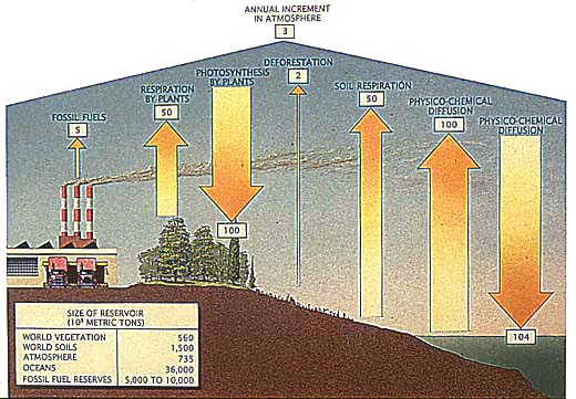
Figure 12. Fluxes and reservoirs for atmospheric carbon.

The correlation between methane, CO₂ and temperature could perhaps be explained by invoking a temperature dependence to the cycling of CO₂ and methane through the environment. Figure 12 shows examples of fluxes and reservoirs for CO₂. The main reservoir is the ocean. A dependence of the flux from the ocean to temperature (the higher the temperature, the greater the flux to the atmosphere) could explain the correlation for CO₂, while a similar temperature dependence for decomposition could explain the methane correlation.

Modern Changes

Modern changes in temperature and carbon dioxide are shown in Figures 13 and 14. Modern methane variations have been shown in Figure 2.

It is clear from these figures that rapid changes are underway - at rates far exceeding anything discussed so far.

It must be assumed that human activities (known as Anthropogenic Effects) are dominating the present changes.

The past century has seen an increase in the global mean temperature of 0.8^oC.

Some of the variations seen are a consequence of volcanic eruptions. Such events can emit large quantities of dust into the stratosphere where sunlight can be intercepted for a period of a few years.

The upward trend may also be a consequence of the increasing levels of carbon dioxide, methane and CFCs put into the atmosphere through various anthropogenic processes.

Figure 15 shows multi-year measurements of carbon dioxide abundances from a single location in Hawaii. The strong yearly signal (peak in winter months, minimum in summer months) can be seen, together with the strong increase due to anthropogenic effects. The causes and consequences of this rise will be the subject of much additional discussion in this course. Figure 16 shows the modern climate records for methane and carbon dioxide. Both species show a strong yearly cycle (peaking in the winter months). The cycle is more pronounced in the Northern Hemisphere due to the preponderance of human activities and continents there.

Figure 13. Modern variations in CO₂ and temperatures.

Figure 14. Recent changes in global mean air temperature. Top panel Northern Hemisphere. Bottom panel Southern Hemisphere.

Figure 15. Multi-year climate record of CO₂ abundances in Hawaii.

Figure 16. Multi-year and latitudinal variation of CO₂ (top) and CH₄ (bottom).

3. Climate Models

The Intergovernmental Panel on Climate Change has released a series of Technical Summaries in 2001. Download:

"Climate Change 2001: The Scientific Basis" (especially germane to this topic)
"Climate Change 2001: Impacts, Adaptation and Vulnerability"
"Climate Change 2001: Mitigation"

A number of sophisticated global climate models have been developed over the past 15 years for the purpose of predicting future climatic change. The most highly developed models are three-dimensional and time dependent and divide the globe up into a series of interacting boxes. The reservoirs and fluxes of importance are coded into the computer program which then solves the conservation equations of mass, momentum, and energy in order to calculate the evolving state of the atmosphere/hydrosphere system.

In general, models such as these must be validated against observations. This is done sometimes by running the model backwards in time to specify past, known climates. However useful, these predictive models have to constantly checked against experimental data to insure accurate results.

Climate models are often used to predict the climate of an Earth in which the carbon dioxide concentration has doubled. This is a prospect very likely to occur within the next 50-100 years, given the current increasing rates of anthropogenic CO₂.

Below are some results of climate models run under twice the current global carbon dioxide concentration.The model predictions for future climate are based on forward estimates of the rate of fossil fuel consumption. They also include prescriptions for the multiple interactions among clouds, land, oceans, etc.:

Climate model predict a climate that is significantly hotter and more humid than now. (Figure 17).
Climate models predict an increase in the mean sea level of 6 meters over the next 100 years. Different scenarios give different results, but the basic trend is the same (Figure 18).
Climate Models also predict increases of 4 degrees over the same 100 year interval. It must be noted that the exact prediction is dependent on the assumptions used for fossil fuel consumption rate (see Figure 19).

Figure 17. Interaction of Climate Models and experimental data.

Figure 18. Climate models predictions for sea level changes
according to several scenarios of fossil fuel comsumption.

Figure 19. Climate model predictions for temperature changes
according to several scenarios of fossil fuel consumption.

4. Summary

A paleoclimate record has been developed using different techniques, stretching back over 2 billion years. The Earth was warmer than at present for most of this time, punctuated by infrequent Ice Ages.
The Great Ice Ages may have been caused by processes associated with continental drift and greenhouse warming.
The interglacial periods are related to orbital changes described by the Milankovitch cycles, among other factors.
In recent times, temperature changes and greenhouse gas abundances are correlated. Rapid global warming is underway and models have been developed to predict the effects of these changes.

Compendium of Trace Gases

In the past twenty years, it has become increasingly evident that certain trace gases play a major role in determining the climate system - far in excess of what might be thought based on their small numbers. Carbon Dioxide is perhaps the principal culprit for potential global warming, but it is by no means the only one.

The above shows the relative contribution to tropospheric warming due to the greenhouse effect of various gases. This plot, taken from model calculations, contains two surprises. Firstly, the Chloro-fluorocarbons (CFC's) taken as a whole (there are several members of this family of gases) represent the second most important gas for global warming - even though their concentrations are measured in the parts per trillion, as opposed to parts per billion for carbon dioxide and methane. The CFC's are entirely of anthropogenic origin.

Secondly, we see that both ozone and nitrous oxide (N2O or "laughing gas") are significant greenhouse gases. In fact, most gases that are made up of three or more atoms are effective greenhouse gases. This is because they have the ability to absorb and emit infra-red radiation via processes of rotational and vibrational excitation (think, for example, of the three atoms making up CO2 as being connected by springs - infra red light is emitted and absorbed in association with the jiggling and spinning of the springed molecule).

For a full study of the issues relating to Global Change, therefore, we need to account quantitatively for the sources and sinks of all these greenhouse gases, incorporating a discussion of the extent to which their presence in the atmosphere can be attributed to human activities and a projection of their future abundances.

Tables 1 and 2 provide more detailed summaries of some of the attributes of important trace gases that are found in the Earth's atmosphere.

Table 1 lists the major anthropogenic sources for each trace gas, as well as the mean residence time and the projected change in abundance with time. The last column of Table 1 provides an estimate for the projected concentration of the gas in the year 2030 in parts per billion (ppb), based on a conservative assumption for future global industrial development.

Table 1. Compendium of Trace Gases in the Atmosphere

GAS	MAJOR ANTHROPOGENIC SOURCES	Anthropogenic Total Emmision /yr(M of Tons)	AVERAGE RESIDENCE TIME IN ATMOSPHERE	AVERAGE CONCENTRATION 100 YEARS AGO (PPB)	APPROXIMATE CURRENT CONCENTRATION (PPB)	PROJECTED CONCENTRATION IN YEAR 2030 (PPB)
CARBON MONOXIDE (CO)	Fossil-Fuel Combustion, Biomass Burning	700/ 2,000	Months	?, N. Hem. 40-80, S. Hem. (Clean Atmospheres)	100-200, N. Hem. 40-80, S. Hem. (Clean Atmospheres)	Probably increasing
CARBON DIOXIDE (CO₂)	Fossil-Fuel Combustion, Deforestation	5,500/ ~5,500	100 Years	290,000	350,000	400,000-550,000
METHANE (CH₄)	Rice Fields, Cattle, Landfills, Fossil -Fuel Production	300-400/ 550	10 Years	900	1,700	2,200-2,500
NO_X GASES	Fossil-Fuel Combustion, Biomass Burning	20-30/ 30-50	Days	.001 to ? (Clean to Industrial)	.001-50 (Clean to Industrial)	.001-50 (Clean to Industrial)
NITROUS OXIDE (N₂O)	Notrogenous Fertilizers, Deforestation, Biomass Burning	6/ 25	170 Years	285	310	330-350
SULFUR DIOXIDE (SO₂)	Fossil-Fuel Combustion, Ore Smelting	100-130/ 150-200	Days to Weeks	.03 to ? (Clean to Industrial)	.03-50 (Clean to Industrial)	.03-50 (Clean to Industrial)
CHLORO- FLUORO- CARBONS	Aerosol Sprays, Refrigerants, Foams	-1/1	60-100 Years	0	About 3 (Chlorine atoms)	2.4-6 (Chlorine atoms)

Table 2 provides information on the two principal concerns we always have when discussing a trace gas, namely:

1.what is its the "Greenhouse Potential" (GP)?
2.what is its the Ozone Depletion Potential (ODP)?

Table 2. Ozone Depletion Potential and Greenhouse Potential for various gases

Trace Gas	Formula	Primary Source	Average Life in Atmosphere (Years)	ODP^*	GP^**
CFC-11	CFCl₃	Refrigerant/AC, Plastic Foams, Aerosols	75	1.0	0.40
CFC-12	CF₂Cl₂	Refrigerant/AC, Plastic Foams, Sterilants	110	1.0	1.00
CFC-113	C₂F₃Cl₃	Solvents	90	0.8	0.3-0.8
Halon 1211	CF₂ClBr	Fire Extinguishers	25	3.0	?
Halon 1301	CF₃Br	Fire Extinguishers	110	10.0	0.80
Carbon Tetrachloride	CCl₄	Industrial Processes	67	1.1	0.05
Methyl Chloroform	CH₃CCl₃	Industrial and Natural Processes	8	0.1	0.01
Nitrous Oxide	N₂O	Fossil Fuels	150	--	0.016
Methane	CH₄	Biogenic Activity, Fossil Fuels	11	--	0.001
Carbon Dioxide	CO₂	Fossil Fuels	7	--	0.00005
Carbon Monoxide	CO	Motor Vehicles	0.4	--	--

^* ozone depletion potential (CFC-11 = 1.0)
^** greenhouse potential (CFC-12 = 1.0)

For convenience, both GP and ODP are measured on a per molecule basis, using as reference the potentials of specific CFC molecules. Thus, for example, we see from Table 2 that a molecule of methane has only 0.001 times the effectiveness of a molecule of CFC-12 for greenhouse warming. Similarly, we see that Carbon Dioxide is not a particularly effective greenhouse gas on a per molecule basis (GP = 0.00005), but since it is much more abundant than the others, it still comes out on top (see Figure 1).

In addition to these gases, clouds and aerosols also play important roles in radiative forcing. A discussion of the physical processes involved in the adsorption and/or scattering of radiation by aerosols and clouds can be found in the relevant GC1 lecture.

Additional information about the Earth’s natural greenhouse and the role played by anthropogenic emissions can be found at the relevant GC1 web page.

References

Climate Change 2001: The Scientific Basis; IPCC 2001
Climate Change 2001: Synthesis Report; IPCC 2001
NRC, Improving the Effectiveness of U.S. Climate Modeling, 2001
J. T. Houghton et al., eds. Climate Change 1995: The Science of Climate Change, published for the IPCC, in collaboration with WMO and UNEP

–

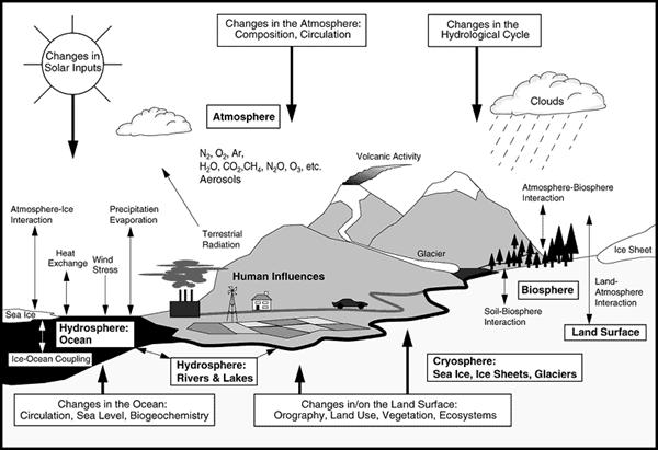
Modeling the Climate System

Climate models

Major components of the climate system must be represented in sub-models (atmosphere, ocean, land surface, cryosphere and biosphere), along with the processes that go on within and between them. General circulation models (GCMs), such as Atmosphere GCMs and Ocean GCMs, include equations that describe the large-scale evolution of momentum, heat and moisture. An important consideration for these models is their resolution, which represents their accuracy. An atmosphere GCM has a resolution of approximately 250 km in the horizontal direction, and an ocean GCM of about 125 - 250 km in the horizontal and about 200 to 400 m in the vertical.

Many physical processes (e.g., related to clouds or ocean convection) take place on much smaller spatial scales than the model grid and therefore cannot be modeled and resolved explicitly. Their average effects are approximately included in a simple way by taking advantage of physically based relationships with the larger-scale variables. This technique is known as parameterization.

Quantitative projections of future climate change require models that simulate all the important processes governing the future evolution of the climate atmosphere, land, ocean and sea ice developed separately and then gradually integrated considerable computing power to run comprehensive "AOGCMs." Simpler models (e.g., coarser resolution and simplified dynamics and physical processes) are widely used to explore different scenarios of emissions of greenhouse gases to assess the effects of assumptions or approximations in model parameters

Together, simple, intermediate, and comprehensive models form a “hierarchy of climate models”, all of which are necessary to explore choices made in parameterizations and assess the robustness of climate changes.

Source: Climate Change 2001: The Scientific Basis; IPCC 2001

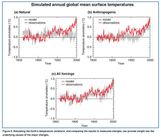
One common test of model accuracy is their ability to predict past temperatures. The following graphs show comparisons of actual temperature data and GCM model predictions of what those temperatures should have been. One main criticism of this approach is that the models themselves were built using past data, and relationships between the variables under consideration could change in the future.

Uncertainty

There are different types of possible uncertainty in climate models. First, there is uncertainty in the quantities used as inputs. The different values are obtained from experiments conducted by different experts, who may disagree about the results. It is difficult to resolve these issues because conflicting data can come from equally well-designed experiments. There is also uncertainty about model structure, or how the data inputs are combined together to form a complete picture. The following bullets summarize primary sources of uncertainty:

Data uncertainties arise from the quality or appropriateness of the data used as inputs to models.
Modeling uncertainties arise from an incomplete understanding of the modeled phenomena, or from approximations that are used in formal representation of the processes.
Completeness uncertainties refer to all omissions due to lack of knowledge. They are, in principle, non-quantifiable and irreducible.

Credibility of Projections

Assessment of the credibility of GCM projections of climate change indicates that there are a number of processes and feedbacks requiring sustained research. These include cloud-radiation-water vapor interactions, ocean circulation and overturning, aerosol forcing, decadal to centennial variability, land-surface processes, short-term variability affecting the frequency and intensity of extreme and high impact events (e.g., monsoons, hurricanes, storm systems), interactions between chemistry and climate change and improved representations of atmospheric chemical interactions within climate models. The image below is a diagram of our current level of understanding of these interactions, which is given to illustrate the complexity of interactions which must be taken into consideration.

Source: Global Environmental Change:Research Pathways for the Next Decade; NRC 1999

Greenhouse Gas (GHG) Emissions

The primary driving forces of greenhouse gas emissions are demographic change, social and economic development, and the rate and direction of technological change.

Emissions Scenarios

Scenarios of emissions are neither predictions nor forecasts; they are alternative images of how the future might unfold. These are used as tools with which to analyze how driving forces may influence future emission outcomes and to assess the associated uncertainties.

Scenarios are given descriptive names and have different part to them. The storyline is a coherent narrative which describes a particular demographic, social, economic, technological, environmental, and policy future. All interpretations and quantifications of one storyline together are called a scenario family. Each scenario family includes a storyline and a number of alternative interpretations and quantifications of each storyline to explore variations of global and regional developments and their implications for greenhouse gas and sulfur emissions. Storylines were formulated in a process that identified driving forces, key uncertainties, possible scenario families, and their logic.

Source: IPCC Special Report on Emissions Scenarios

Scenarios also have uncertainties associated with them. The sources of these uncertainties include the choice of storylines and the authors' interpretation of those storylines. Another important source of uncertainty is the translation of the understanding of linkages between driving forces into quantitative inputs for scenario analysis. Furthermore, there are differences in methodology, sources of data, and inherent uncertainties which result from assumptions made to simplify models. Now let us look at the actual scenarios in detail:

A1 Storyline and Scenario Family

These assume a world with very rapid economic growth, low population growth, and rapid introduction of new and more efficient technologies. The major underlying themes are convergence among regions, capacity building, increased cultural and social interactions, and substantial reduction in regional differences in per capita income.

Alternative directions of technological change are represented as A1FI (high coal, oil and gas), A1B (balanced, or even distribution among options) and A1T (predominantly non-fossil fuel).

· A2 Storyline and Scenario Family

A highly heterogeneous world with: high population growth (due to slow convergence of fertility patterns across regions), regionally-oriented economic development, per capita economic growth, and more fragmented/slower technological change. The major underlying themes are self reliance preservation of local identities.

· B1 Storyline and Scenario Family

A convergent world with: rapid changes in economic structures toward a service and information economy, low population growth (same as A1), reductions in material intensity, and introduction of clean and resource-efficient technologies. Major Underlying Themes are the global solutions to economic, social, and environmental sustainability (without additional climate initiatives), as well as improved equity.

· B2 Storyline and Scenario Family

A world with: intermediate levels of economic development, moderate population growth, reductions in material intensity, and less rapid and more diverse technological change. Major Underlying Themes are local solutions to economic, social, and environmental sustainability (without additional climate initiatives), social equity (with local/regional focus), and environmental protection (with local/regional focus).

The following chart is a summary of the qualitative directions of these scenarios for different indicators:

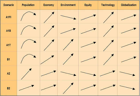
Source: Climate Change 2001 Mitigation Technical Summary

Now compare the chart above to the next set of graphs, which contain predictions for the global climate based on the above assumptions:

Anthropogenic emissions of Greenhouse Gases Under Different Scenarios

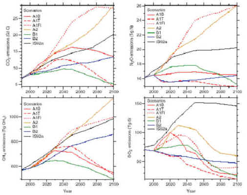
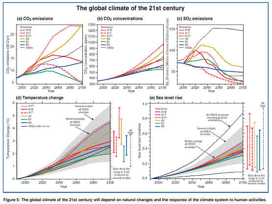
Source: Working Group I Summary for Policy Makers; IPCC 2001

The Potential Impacts of Climate Change on the United States

We wish to learn:

In what ways is the United States vulnerable to climate variability and change?
What steps can be taken to contribute to sustainable solutions to the greenhouse problem?

The Global Change Research Act of 1990 [Public Law 101-606] highlighted early scientific findings that human activities were starting to change the global climate. It found that:

“(1) Industrial, agricultural, and other human activities, coupled with an expanding world population, are contributing to processes of global change that may significantly alter the Earth habitat within a few generations;

(2) Such human-induced changes, in conjunction with natural fluctuations, may lead to significant global warming and thus alter world climate patterns and increase global sea levels. Over the next century, these consequences could adversely affect world agricultural and marine production, coastal habitability, biological diversity, human health, and global economic and social well-being.”

Congress established the US Global Change Research Program (USGCRP) to address these issues, and mandated that the USGCRP:

“ shall prepare and submit to the President and the Congress an assessment which
integrates, evaluates, and interprets the findings of the Program and discusses the scientific uncertainties associated with such findings;

analyzes the effects of global change on the natural environment, agriculture, energy production and use, land and water resources, transportation, human health and welfare, human social systems, and biological diversity; and analyzes current trends in global change, both human-induced and natural, and projects major trends for the subsequent 25 to100 years.

A National Assessment Synthesis Team (NAST), comprised of government, academic, industry, and non-government organization experts, was formed, and NAST, in collaboration with the Federal agencies that make up the USGCRP, completed an assessment of the potential consequences of climate variability and change on the United States. The results of the assessment were provided in the form of two reports, a Foundation Report, and an Assessment Overview. Cambridge University Press published both reports in 2000.

The focus of NAST, in this first assessment for the United States, was on geographic regions (Northeast, Southeast, Midwest, Great Plains, West, Pacific Northwest, Alaska, and the Islands of the Caribbean and the Pacific) and on sectors (water, agriculture, forests, coastal areas and marine resources, and human health). The assessment team also attempted to identify potential adaptation measures, although there were insufficient resources to complete an evaluation of their costs, practicality or effectiveness. The NAST used state of the science climate models to generate a variety of climate change scenarios (plausible alternative futures) and hydrologic, ecological and socioeconomic system models to assess responses to the different scenarios. It is common to vary such parameters as population and economic growth, and technological development. They also used historical climate records to assess regional and sector sensitivity to climate variability and extremes and to learn about how adaptation occurred in the past. They also completed a number of studies to determine the extent to which the climate would have to change in order for major regional and sector impacts to occur (e.g., the extent to which temperature would have to increase to cause a negative effect on soybeans in the South).

Assumptions

The NAST used two state-of-the-science climate models from the Hadley Centre in the United Kingdom and the Canadian Centre for Climate Modeling and Analysis and data from historical observations to generate a variety of climate scenarios. Both assume mid-range emissions and no major changes in policies to limit the emissions of greenhouse gases. They also assume that, by the year 2100: world population will increase to about 11 billion people; the global economy will continue to grow at about the current average rate, which translates to an increase of more than a factor of 10; increased use of fossil fuels will result in an atmospheric CO2 level of just over 700 ppmv and increased SO2 emissions; and total energy produced each year from non-fossil sources will increase more than 10 times, to provide > 40% of the world’s energy needs. The NAST emissions projections fall in the middle of other Intergovernmental Panel for Climate Change (IPCC) emissions scenarios.

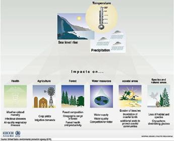
Sector Overview

The NAST decided to focus on five issues of national importance: agriculture, water, human health, coastal areas and marine resources, and forests. The key issues identified for the agriculture sector are crop yield changes and associated economic consequences, changing water demands for irrigation, surface water quality, increasing pesticide use, and climate variability. The key issues identified for the water sector are competition for water supplies, surface water quantity and quality, groundwater quantity and quality, floods, droughts, and extreme precipitation events, and ecosystem vulnerabilities. The key issues identified for the health sector are temperature-related illnesses and deaths, health effects related to extreme weather events, air pollution-related health effects, water- and food-borne diseases, and insect-, tick-, and rodent-borne diseases. The key issues identified for the coastal areas and marine resources sector are shoreline erosion and human communities, threats to estuarine health, coastal wetland survival, coral reef die-offs, and stresses on marine fisheries. The key issues identified for the forest sector are effects on forest productivity, natural disturbances such as fire and drought, biodiversity changes, and socioeconomic impacts.

The assessment concludes that:

Agriculture: “Overall productivity of American agriculture will likely remain high, and is projected to increase throughout the 21st century, with northern regions faring better than southern ones. Though agriculture is highly dependent on climate, it is also highly adaptive. Weather extremes, pests, and weeds will likely present challenges in a changing climate. Falling commodity prices and competitive pressures are likely to stress farmers and rural communities.”

Water: “Rising temperatures and greater precipitation are likely to lead to more evaporation and greater swings between wet and dry conditions. Changes in the amount and timing of rain, snow, runoff, and soil moisture are very likely. Water management, including pricing and allocation, will very likely be important in determining many impacts.”

Human Health: “Heat-related illnesses and deaths, air pollution, injuries and deaths from extreme weather events, and diseases carried by water, food, insects, ticks, and rodents have all been raised as concerns for the US in a warmer world. Modern public health efforts will be important in identifying and adapting to these potential impacts.”

Coastal Areas and Marine Resources: “Coastal wetlands and shorelines are vulnerable to sea-level rise and storm surges, especially when climate impacts are combined with the growing stresses of increasing human population and development. It is likely that coastal communities will be increasingly affected by extreme events. The negative impacts on natural ecosystems are very likely to increase.”

Forests: “Rising CO2 concentrations and modest warming are likely to increase forest productivity in many regions. With larger increases in temperature, increased drought is likely to reduce forest productivity in some regions, notably in the Southeast and Northwest. Climate change is likely to cause shifts in species ranges as well as large changes in disturbances such a fire and pests”

KEY FINDINGS FROM THE NAST ASSESSMENT

1. Increased warming
Assuming continued growth in world greenhouse gas emissions, the primary climate models used in this Assessment project that temperatures in the US will rise 5-9ºF (3-5ºC) on average in the next 100 years.. A wider range of outcomes is possible.

2. Differing regional impacts
Climate change will vary widely across the US. Temperature increases will vary somewhat from one region to the next. Heavy and extreme precipitation events are likely to become more frequent, yet some regions will get drier. The potential impacts of climate change will also vary widely across the nation.

3. Vulnerable ecosystems
Many ecosystems are highly vulnerable to the projected rate and magnitude of climate change. A few, such as alpine meadows in the Rocky Mountains and some barrier islands, are likely to disappear entirely in some areas. Others, such as forests of the Southeast, are likely to experience major species shifts or break up into a mosaic of grasslands, woodlands, and forests. The goods and services lost through the disappearance or fragmentation of certain ecosystems are likely to be costly or impossible to replace.

4. Widespread water concerns
Water is an issue in every region, but the nature of the vulnerabilities varies. Drought is an important concern in every region. Floods and water quality are concerns in many regions. Snowpack changes are especially important in the West, Pacific Northwest, and Alaska.

5. Secure food supply
At the national level, the agriculture sector is likely to be able to adapt to climate change. Overall, US crop productivity is very likely to increase over the next few decades, but the gains will not be uniform across the nation. Falling prices and competitive pressures are very likely to stress some farmers, while benefiting consumers.

6. Near-term increase in forest growth
Forest productivity is likely to increase over the next several decades in some areas as trees respond to higher carbon dioxide levels. Over the longer term, changes in larger-scale processes such as fire, insects, droughts, and disease will possibly decrease forest productivity. In addition, climate change is likely to cause long-term shifts in forest species, such as sugar maples moving north out of the US.

7. Increased damage in coastal and permafrost areas
Climate change and the resulting rise in sea level are likely to exacerbate threats to buildings, roads, powerlines, and other infrastructure in climatically sensitive places. For example, infrastructure damage is related to permafrost melting in Alaska, and to sea-level rise and storm surge in low-lying coastal areas.

8. Adaptation determines health outcomes
A range of negative health impacts is possible from climate change, but adaptation is likely to help protect much of the US population. Maintaining our nation's public health and community infrastructure, from water treatment systems to emergency shelters, will be important for minimizing the impacts of water-borne diseases, heat stress, air pollution, extreme weather events, and diseases transmitted by insects, ticks, and rodents.

9. Other stresses magnified by climate change
Climate change will very likely magnify the cumulative impacts of other stresses, such as air and water pollution and habitat destruction due to human development patterns. For some systems, such as coral reefs, the combined effects of climate change and other stresses are very likely to exceed a critical threshold, bringing large, possibly irreversible impacts.

10. Uncertainties remain and surprises are expected
Significant uncertainties remain in the science underlying regional climate changes and their impacts. Further research would improve understanding and our ability to project societal and ecosystem impacts, and provide the public with additional useful information about options for adaptation. However, it is likely that some aspects and impacts of climate change will be totally unanticipated as complex systems respond to ongoing climate change in unforeseeable ways.

Source: Climate Change Impacts on the United States, NAST Overview, 2000.

Several issues that are shared by a number of geographic regions were identified. Concerns regarding water are widespread and provide an excellent example of the need for and importance of the adoption of adaptive strategies in the area of water resources.

The following table addresses concerns regarding flooding, drought, loss of snowpack, groundwater quantity and quality, freshwater resources and water quality.

Water Issues in the United States

Region	Floods	Drought	Snowpack/Snowcover	Groundwater	Lake, river, and reservoir levels	Quality
Northeast	x	x	x	x		x
Southeast	x	x		x	x
Midwest	x	x	x	x	x	x
Great Plains	x	x	x	x	x	x
West
Northwest	x	x	x		x
Alaska		x	x
Islands	x	x		x	x

Source: Climate Change Impacts on the United States: The Potential Consequences of Climate Variability and Change, National Assessment Overview, Cambridge University Press, 2000.

As well, a many of the US’s ecosystems face potentially disruptive climate changes. Concerns regarding forests, grasslands, semi-arid and arid regions, tundra, freshwater ecosystems, and coastal and marine ecosystems are shared by a number of regions as shown in the following table.

Ecosystem Type	Impacts	NE	SE	MW	GP	W	NW	AL	IS
Forests	Changes in tree species composition and alteration of animal habitat	X	X	X		X	X	X	X
	Displacement of forests by open woodlands and grasslands under a warmer climate in which soils are drier	X
Grasslands	Displacement of grasslands by open woodlands and forests under a wetter climate					X
	Increase in success of non-native invasive plant species				X	X	X		X
Semi-arid and Arid	Increase in woody species and loss of desert species under wetter climate					X
Tundra	Loss of alpine meadows as their species are displaced by lower-elevation species	X				X	X	X
	Loss of northern tundra as trees migrate poleward							X
	Changes in plant community composition and alteration of animal habitat							X
Freshwater	Loss of prairie potholes with more frequent drought conditions	X	X		X	X	X
	Habitat changes in rivers and lakes as amount and timing of runoff changes and water temperatures rise	X	X	X	X	X	X
Coastal & Marine	Loss of coastal wetlands as sea level rises and coastal development prevents landward migration	X	X			X	X		X
	Loss of barrier islands as sea-level rise prevents landward migration	X	X
	Changes in quantity and quality of freshwater delivery to estuaries and bays alter plant and animal habitat	X	X			X	X	X	X
	Loss of coral reefs as water temperature increases		X						X
	Changes in ice location and duration alter marine mammal habitat							X

Source: Climate Change Impacts on the United States: The Potential Consequences of Climate Variability and Change, National Assessment Overview, Cambridge University Press, 2000.

Although an evaluation of the practicality or feasibility of adaptation strategies was not the focus of this assessment, the NAST did provide the following recommendations:

1. Develop a more integrated approach to examining impacts and vulnerabilities to multiple stresses;

2. Develop new ways to assess the significance of global change to people;

3. Improve projections of how ecosystems will respond;

4. Enchance knowledge of how societal and economic systems will respond to a changing climate and environment;

5. Refine our ability to project how climate will change;

6. Extend capabilities for providing climate information. They also defined a number of areas that could provide needed information in the near term, as listed in the box below.

Areas with High Potential for Providing Needed Information in the Near-Term

· Expand the national capability to develop integrated, regional approaches of assessing the impacts of multiple stresses, perhaps beginning with several case studies.

· Develop capability to perform large-scale (over an acre) whole-ecosystem experiments that vary both CO2 and climate.

· Incorporate representations of actual land cover and land use into models of ecosystem responses.

· Identify potential adaptation options and develop information about their costs, efficacy, side effects, practicality, and implementation.

· Develop better ways to assign values to possible future changes in resources and ecosystems, especially for large changes and for processes and service that do not produce marketable goods.

· Improve climate projections by providing dedicated computer capability for conducting ensemble climate simulations for multiple emission scenarios.

· Focus additional attention on research and analysis of the potential for future changes in severe weather, extreme events, and seasonal to interannual variability.

· Improve long-term data sets of the regional patterns and timing of past changes in climate across the US, and make these data-sets more accessable.

· Develop a set of baseline indicators and measures of environmental conditions that can be used to track the effects of changes in climate.

· Develop additional methods for representing, analyzing, and reporting scientific uncertainties related to global change.

Source: Climate Change Impacts on the United States, Assessment Overview, 2000.