Climates of the Past and Present
Climate Temperature from Ice Cores
Climate Temperatures from Ocean
Sediments
Limitations in Reconstructing
Paleoclimates
1. Paleoclimates
Figure 1. Glaciation in
From abundant geological evidence,
we know that only three hundred and fifty years ago, the world was in the
depths of a prolonged cold spell called the "Little Ice Age," which
lingered for nearly 500 years. Fifty thousand years ago, in the middle of the
last glacial period, large continental ice sheets covered much of North
America, Northern Europe, and
The speed at which climate can
change has also recently become clear: Transitions between fundamentally
different climates can occur within only decades. In order to understand these
variations, we need to reconstruct them over a wide range of temporal and
geographical scales. The importance of this task is underlined by the growing
awareness of how profoundly human activity is affecting climate. As with so
many other complex systems, the key to predicting the future lies in
understanding the past
We need to ask several questions:
What happened? Why did it happen? Has it happened before? Will is happen again?
How do we know about it in the first place? Click the image to the right to explore the
hypothesized changes in ice cover and vegetation.
Paleoclimatology
This is the study of past
climates. It is a fascinating, multidisciplinary field, combining history, anthropology,
archaeology, chemistry, physics, geology, atmospheric, and ocean sciences.
Clues about past climate conditions are obtained from proxy indicators,
types of evidence that can be used to infer climate. These include:
- Isotopic Geochemical Studies: The study of rock
isotopic ratios, ice core bubbles, etc.
- Dendochronology: the study of tree rings
- Pollen Distribution: the study of plant types and
prevalence
- Coral Bed Rings
- Fossils: Studies of geological settings, etc.
- Historical documents, paintings, etc.
Isotope Geochemistry
The most important of these for
the study of long term change involves isotope geochemistry. We have already discussed
the importance of isotopes for rock dating purposes; the carbon14
radiometric technique, for example, can date as far back as 60,000 years.
However, there is another important use of isotopic ratio measurements using
oxygen that is not dependent on radioactivity, but rather on the interaction
between life processes and isotopes.
Oxygen is composed of 8 protons,
and its most common form as 8 neutrons, giving it an atomic weight of 16 (O16)
and is also known a "light" oxygen. A small fraction of oxygen atoms
have 2 extra neutrons and a resulting atomic weight of 18 (O18),
known as "heavy" oxygen. O18, is
a rare form, with about 1 in 500 atoms of O being heavy.
The ratio of these two oxygen
isotopes has changed over the ages and these changes are a proxy to changing
climate in two ways:
Climate Temperature from Ice Cores
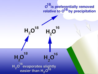
Figure 2. Light oxygen in water (H2O16)
evaporates more readily that water with heavy oxygen (H2O18).
Hence oceans will be relatively rich in O18 when glaciers grow and hold
the precipitated O16.
Ice in glaciers has an increased
proportional abundance of heavy oxygen if it was deposited during relatively
warm periods. To understand why this might be so, we need to think about the
process of glacier formation. The water-ice in glaciers originally came from
the oceans as vapor, later falling as snow and becoming compacted in ice. When
water evaporates, the heavy water (H2O18) is left behind
and the water vapor is enriched in light water (H2O16).
This is simply because it is harder for the heavier molecules to overcome the
barriers to evaporation. Thus, glaciers are relatively enhanced in O16,
while the oceans are relatively enriched in O18. This imbalance is
more marked for colder climates than for warmer climates. In fact, it has been
shown that a decrease of one part per million O18 in ice reflects a
1.5°C drop in air temperature at the time it originally evaporated from the
oceans.
While there are complexities with
the analysis, a simple measurement of the isotopic ratio of O18 in
ice cores can be directly related to climate. Ice cores from
Climate Temperatures from Ocean
Sediments
Shells of dead marine organisms
are made up of calcium carbonate (CaCO3). The oxygen in the
carbonate reflects the isotopic abundance in the shallow waters where the
creatures lived. Thus if we can find and date ever more ancient sediments made
up of old sea shells, we can determine the isotopic ratio of oxygen and infer
the sea surface temperature at that time. The more O18
found in the sediment, the colder the climate (inverse relationship to that of
glacier ice).
Many ice cores and sediment cores
have been drilled in Greenland,
Figure 3. Changes in
temperature as deduced using a number of paleoclimate
techniques, each representing different time periods and/or regions.
Other Proxy Indicators
Figure 3 summarizes the climate
record as presently understood and lists some of the techniques used for the
measurement.
The most commonly used indicators include
pollen, faunal and floral remains, sediment types or composition and geomorphological features indicating physical conditions.
In the ocean, indicators such as microplankton,
pollen, and sediments settle to the sea floor, where they accumulate to provide
a nearly continuous record of climate for millions of years.
The bottom panel shows the record
for the last million years. Each successively higher panel expands the shaded
part of the panel immediately below. The top panel summarizes the last century.
Animations of the Temperature
Record from 1856 to 1997 are available to explore
spatial trends in temperature.
Limitations in Reconstructing Paleoclimates
The limitations in this process
result from uncertainties associated with dating the proxy indicators or other
evidence. There are two fundamental types of dating:
- Absolute dating
Techniques that identify the actual geological time represented by the evidence. Techniques are limited and rely predominately on evaluating the amount of decay of naturally occurring radioactive isotopes. - Relative dating
Techniques that are able to differentiate time relative to other points in time. Stratigraphy establishes a relative sequence of events or characteristics within which the evidence lies. If this same sequence can be identified in multiple locations it can be used to establish the relationship between locations and the relative timing of the indicators.
2. Current Climate
Climate differs from weather in
that it provides a statistical view of seasonal and daily weather events over a
long term period. Thus, for example, the passage of a frontal system over
Climate records are most often
expressed in terms of temperatures, winds, precipitation, and pressures - all
parameters that can be measured at multiple sites around the globe. Over the
years a large data base of weather event measurements has been obtained,
leading to a good description of today's climate.
We find that climate varies widely
around the globe - we have deserts and rain forests, ice caps and "death
valleys". As for most subjects discussed in this course, there is a taxonomy of sub-disciplines and we can speak of the
following:
Figure 4.
- Microclimate: climate conditions near the
surface over distances of a few meters. Great perturbations to the
microclimate can rapidly affect plant life.
- Mesoclimate: climate conditions over a
few square kilometers, for example, climate of a town, valley, beach, etc.
- Macroclimate: climate conditions for a
state or a country - over scales ~1000 km or greater.
- Global Climate: The overall climate of the
planet. We have already discussed, for example, the mean surface temperature
and its variations with geologic time.
The many factors that control
local climates include: intensity of overhead sun - including its latitudinal
variation; the distribution of land and water; ocean currents; prevailing winds;
positions of semi-permanent high- and low-pressure areas; mountain barriers;
altitude. The effects of these controls can be seen in global patterns of
temperature and precipitation. Examples of local climatic data are shown in
Figure 4. These graphs are derived from temperature and precipitation data available from the
Great differences in climate occur
from place to place, even within the continental
Figures 5 uses this system to
provide a summary of the types of climates found on today's Earth.
TABLE 1. Climatological monthly temperatures
and precipitation for
|
|
JAN |
FEB |
MAR |
APR |
MAY |
JUN |
JUL |
AUG |
SEP |
OCT |
NOV |
DEC |
ANNUAL |
|
Temperature (°F) |
22.9 |
25.4 |
35.7 |
47.3 |
58.4 |
67.6 |
72.3 |
70.5 |
63.2 |
51.2 |
40.2 |
28.3 |
48.6 (MEAN) |
|
Precipitation (in) |
1.76 |
1.74 |
2.55 |
2.95 |
2.92 |
3.61 |
3.18 |
3.43 |
2.89 |
2.10 |
2.67 |
2.82 |
32.62 (TOTAL) |
|
Data from the National Climate Data Center |
|||||||||||||
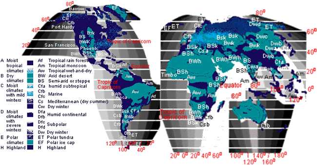
Figure 4
Global Temperatures
Figure 5. Average annual sea level temperatures
throughout the world (degrees F)
Up to
now, we have discussed the global average temperature. Actual local temperatures
can differ greatly from the global mean, being generally warmer at lower
latitudes and colder at higher latitudes. Figure 5 illustrates the annual sea
level temperature (in degrees F). The lines are contours of temperature (called
isotherms) and are generally oriented east-west. The primary changes are in
latitude, with the equatorial region being the hottest due to the extra
sunlight absorbed there.
Note how the isotherms tend to
bend along coastlines. This is due to the unequal heating of land and water and
the tendency of the winds to blow along coastlines. Also of significance are
the ocean currents and the upwelling of cold deep ocean waters. Examples of
ocean currents include the California Current which flows southwards along the
Californian coast and the Gulf Stream which flows northwards in the
The Atmosphere in Motion
One of the more important factors
for climate is the global wind system. Winds are driven into motion by forces
on the air. There is a system of prevailing winds whose purpose it is to
transfer the excess energy received at low latitudes to high latitudes. If the
earth did not rotate and did not have any continental land masses, then the
wind system would be rather simple.
Figure 6. Wind patterns of the world for (A) a hypothetical world with no
rotation,
(B) the world with rotation, and (C) the resulting bands of general circulation.
The excess heat received in the
equatorial region would cause the air to rise and blow away towards higher
latitudes. In order for air to be conserved, the outward motion at high
latitudes near the equator has to be balanced by inward low altitude winds.
This system is a huge twin-cell circulation pattern (one cell in each
atmosphere). These idealized cells are called Hadley Cells.
Because the earth rotates and has
continental land masses, the actual prevailing winds do not directly blow from
pole to equator as in but rather curve around and form a multicellular
circulation pattern. The curving form the initial direction of the winds is
called the "Coriolis effect" and is due to
rotation. The curvature is so great as to split up each Hadley cell into three
smaller cells.
The highest temperatures occur in
the subtropical deserts, e.g., the African Sahara. The lowest mean temperatures
occur in
It is interesting to note here an
important feedback process that can occur at high latitudes. In very cold
regions, such as
Global Precipitation
Figure 7 summarizes the modern
global mean precipitation climate record. Notice the high degree of regional
variability.
Figure 7. Global patterns of precipitation
are closely tied to general circulation and topographic changes
Current Trends
The global average surface temperature
has increased by 0.6 ±0.2°C since the late 19th century (IPCC,
2001). It is very likely that the 1990s was the warmest decade and 1998 the
warmest year in the instrumental record since 1861 (see Figure 8).
As indicated in Figure 8, most of the increase in global
temperature since the late 19th century has occurred in two distinct periods: 1910
to 1945 and since 1976. The rate of increase of temperature for both periods is
about 0.15°C/decade. Recent warming has been greater over land compared to
oceans; the increase in sea surface temperature over the period 1950 to 1993 is
about half that of the mean land-surface air temperature. The high global
temperature associated with the 1997 to 1998 El Niño event stands out as an
extreme event, even taking into account the recent rate of warming.
Figure 8: Combined annual land-surface air
and sea surface temperature anomalies (°C) 1861 to 2000, relative to 1961 to
1990. Two standard error uncertainties are shown as bars on the annual number
[from IPCC, 2001]
It also appears that the spatial
patterns of warming that occurred in the early part of the 20th century were
different than those that occurred in the latter part. Figure 9 shows the regional patterns of the
warming that have occurred over the full 20th century, as well as for three
component time periods. The most recent period of warming (1976 to 1999) has
been almost global, but the largest increases in temperature have occurred over
the mid- and high latitudes of the continents in the Northern Hemisphere.
Year-round cooling is evident in the northwestern North Atlantic and the
central
| 1901-2000 |
| 1910-1945 | 1946-1975 | 1976-2000 |
Figure 9. Temperature trends for the periods 1901-1999, 1910-1945, 1946-1975
and 1976-1999. Trends are represented by the area of the circle with red
representing increases, blue representing decreases, and green little or no
change. [From IPCC, 2001]
4. Summary
- The Earth's climate has changed dramatically in the
past, apparently in response to natural changes in orbital characteristics
and topography.
- We are able to deduce past climates through multiple
techniques but much of the progress in resolving Cenozoic climate change
has resulted from oxygen and carbon isotope records.
- The climate of the Earth today varies by latitude
and, to a lesser degree, longitude and is controlled by varying solar
radiation availability and the redistribution of energy through wind and
currents.