and the first three steps were discussed in detail. The composition of the present atmosphere however required the formation of oxygen to sufficient levels to sustain life, and required life to create the sufficient levels of oxygen. This era of evolution of the atmosphere is called the "Biological Era."

The Biological Era - The Formation of Atmospheric Oxygen

The biological era was marked by the simultaneous decrease in atmospheric carbon dioxide (CO₂) and the increase in oxygen (O₂) due to life processes. We need to understand how photosynthesis could have led to maintenance of the ~20% present-day level of O₂.

The build up of oxygen had three major consequences that we should note here.

Firstly, Eukaryotic metabolism could only have begun once the level of oxygen had built up to about 0.2%, or ~1% of its present abundance. This must have occurred by ~2 billion years ago, according to the fossil record. Thus, the eukaryotes came about as a consequence of the long, steady, but less efficient earlier photosynthesis carried out by Prokaryotes.

Oxygen through photolysis
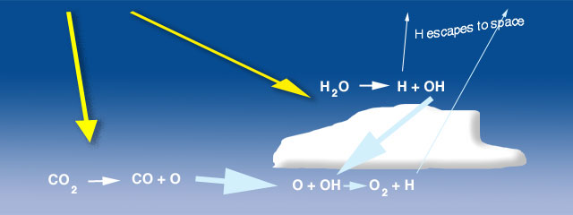
Figure 1. Photolysis of water vapor and carbon dioxide produce hydroxyl and atomic oxygen, respectively, that, in turn, produce oxygen in small concentrations. This process produced oxygen for the early atmosphere before photosynthesis became dominant.

Oxygen increased in stages, first through photolysis (Figure 1) of water vapor and carbon dioxide by ultraviolet energy and, possibly, lightning:

H₂O -> H + OH

produces a hydroxyl radiacal (OH) and

CO₂ -> CO+ O

produces an atomic oxygen (O). The OH is very reactive and combines with the O

O + OH -> O₂ + H

The hydrogen atoms formed in these reactions are light and some small fraction excape to space allowing the O2 to build to a very low concentration, probably yielded only about 1% of the oxygen available today.

Secondly, once sufficient oxygen had accumulated in the stratosphere, it was acted on by sunlight to form ozone, which allowed colonization of the land. The first evidence for vascular plant colonization of the land dates back to ~400 million years ago.

Thirdly, the availability of oxygen enabled a diversification of metabolic pathways, leading to a great increase in efficiency. The bulk of the oxygen formed once life began on the planet, principally through the process of photosynthesis:

6CO₂ + 6H₂O <--> C₆H₁₂O₆ + 6O₂

where carbon dioxide and water vapor, in the presence of light, produce organics and oxygen. The reaction can go either way as in the case of respiration or decay the organic matter takes up oxygen to form carbon dioxide and water vapor.

Life started to have a major impact on the environment once photosynthetic organisms evolved. These organisms fed off atmospheric carbon dioxide and converted much of it into marine sediments consisting of the innumerable shells and decomposed remnants of sea creatures.

Cumulative history of O₂ by photosynthesis through geologic time.

While photosynthetic life reduced the carbon dioxide content of the atmosphere, it also started to produce oxygen. The oxygen did not build up in the atmosphere for a long time, since it was absorbed by rocks that could be easily oxidized (rusted). To this day, most of the oxygen produced over time is locked up in the ancient "banded rock" and "red bed" rock formations found in ancient sedimentary rock. It was not until ~1 billion years ago that the reservoirs of oxidizable rock became saturated and the free oxygen stayed in the air. The figure illustrates a possible scenario.

We have briefly mentioned the difference between reducing (electron-rich) and oxidizing (electron hungry) substances. Oxygen is the most important example of the latter type of substance that led to the term oxidation for the process of transferring electrons from reducing to oxidizing materials. This consideration is important for our discussion of atmospheric evolution, since the oxygen produced by early photosynthesis must have readily combined with any available reducing substance. It did not have far to look!

We have been able to outline the steps in the long drawn out process of producing present-day levels of oxygen in the atmosphere. We refer here to the geological evidence.

Banded Iron Formations

When the oceans first formed, the waters must have dissolved enormous quantities of reducing iron ions, such as Fe²⁺. These ferrous ions were the consequences of millions of years of rock weathering in an anaerobic (oxygen-free) environment. The first oxygen produced in the oceans by the early prokaryotic cells would have quickly been taken up in oxidizing reactions with dissolved iron. This oceanic oxidization reaction produces Ferric oxide Fe₂O₃ that would have deposited in ocean floor sediments. The earliest evidence of this process dates back to the Banded Iron Formations, which reach a peak occurrence in metamorphosed sedimentary rock at least 3.5 billion years old. Most of the major economic deposits of iron ore are from Banded Iron formations. These formations, were created as sediments in ancient oceans and are found in rocks in the range 2 - 3.5 billion years old. Very few banded iron formations have been found with more recent dates, suggesting that the continued production of oxygen had finally exhausted the capability of the dissolved iron ions reservoir. At this point another process started to take up the available oxygen.

Red Beds

Once the ocean reservoir had been exhausted, the newly created oxygen found another large reservoir - reduced minerals available on the barren land. Oxidization of reduced minerals, such as pyrite FeS₂ , exposed on land would transfer oxidized substances to rivers and out to the oceans via river flow. Deposits of Fe₂O₃ that are found in alternating layers with other sediments of land origin are known as Red Beds, and are found to date from 2.0 billion years ago. The earliest occurrence of red beds is roughly simultaneous with the disappearance of the banded iron formation, further evidence that the oceans were cleared of reduced metals before O₂ began to diffuse into the atmosphere.

Finally after another 1.5 billion years or so, the red bed reservoir became exhausted too (although it is continually being regenerated through weathering) and oxygen finally started to accumulate in the atmosphere itself. This signal event initiated eukaryotic cell development, land colonization, and species diversification. Perhaps this period rivals differentiation as the most important event in Earth history.

The oxygen built up to today's value only after the colonization of land by green plants, leading to efficient and ubiquitous photosynthesis. The current level of 20% seems stable.

The Oxygen Concentration Problem.

Why does present-day oxygen sit at 20%? This is not a trivial question since significantly lower or higher levels would be damaging to life. If we had < 15% oxygen, fires would not burn, yet at > 25% oxygen, even wet organic matter would burn freely.

The Early Ultraviolet Problem

The genetic materials of cells (DNA) is highly susceptible to damage by ultraviolet light at wavelengths near 0.25 µm. It is estimated that typical contemporary microorganisms would be killed in a matter of seconds if exposed to the full intensity of solar radiation at these wavelength. Today, of course, such organisms are protected by the atmospheric ozone layer that effectively absorbs light at these short wavelengths, but what happened in the early Earth prior to the significant production of atmospheric oxygen? There is no problem for the original non-photosynthetic microorganisms that could quite happily have lived in the deep ocean and in muds, well hidden from sunlight. But for the early photosynthetic prokaryotes, it must have been a matter of life and death.

It is a classical "chicken and egg" problem. In order to become photosynthetic, early microorganisms must have had access to sunlight, yet they must have also had protection against the UV radiation. The oceans only provide limited protection. Since water does not absorb very strongly in the ultraviolet a depth of several tens of meters is needed for full UV protection. Perhaps the organisms used a protective layer of the dead bodies of their brethren. Perhaps this is the origin of the stromatolites - algal mats that would have provided adequate protection for those organisms buried a few millimeters in. Perhaps the early organisms had a protective UV-absorbing case made up of disposable DNA - there is some intriguing evidence of unused modern elaborate repair mechanisms that allow certain cells to repair moderate UV damage to their DNA. However it was accomplished, we know that natural selection worked in favor of the photosynthetic microorganisms, leading to further diversification.

Fluctuations in Oxygen

The history of macroscopic life on Earth is divided into three great eras: the Paleozoic, Mesozoic and Cenozoic. Each era is then divided into periods. The latter half of the Paleozoic era, includes the Devonian period, which ended about 360 million years ago, the Carboniferous period, which ended about 280 million years ago, and the Permian period, which ended about 250 million years ago.

According to recently developed geochemical models, oxygen levels are believed to have climbed to a maximum of 35 percent and then dropped to a low of 15 percent during a 120-million-year period that ended in a mass extinction at the end of the Permian. Such a jump in oxygen would have had dramatic biological consequences by enhancing diffusion-dependent processes such as respiration, allowing insects such as dragonflies, centipedes, scorpions and spiders to grow to very large sizes. Fossil records indicate, for example, that one species of dragonfly had a wing span of 2 1/2 feet.

Geochemical models indicate that near the close of the Paleozoic era, during the Permian period, global atmospheric oxygen levels dropped to about 15 percent, lower that the current atmospheric level of 21 percent. The Permian period is marked by one of the greatest extinctions of both land and aquatic animals, including the giant dragonflies. But it is not believed that the drop in oxygen played a significant role in causing the extinction. Some creatures that became specially adapted to living in an oxygen-rich environment, such as the large flying insects and other giant arthropods, however, may have been unable to survive when the oxygen atmosphere underwent dramatic change.

2. Composition of the Present Atmosphere

Comparison to Other Planets

The overall composition of the earth's atmosphere is summarized below along with a comparison to the atmospheres on Venus and Mars - our closest neighbors.

	VENUS	EARTH	MARS
SURFACE PRESSURE	100,000 mb	1,000 mb	6 mb
	*COMPOSITION*
CO₂	>98%	0.03%	96%
N₂	1%	78%	2.5%
Ar	1%	1%	1.5%
O₂	0.0%	21%	2.5%
H₂O	0.0%	0.1%	0-0.1%
	(more on Mars)	(more on Earth)	(more on Mars)

The variations in concentration from the Earth to Mars and Venus result from the different processes that influenced the development of each atmosphere. While Venus is too warm and Mars is too cold for liquid water the Earth is at just such a distance from the Sun that water was able to form in all three phases, gaseous, liquid and solid. Through condensation the water vapor in our atmosphere was removed over time to form the oceans. Additionally, because carbon dioxide is slightly soluble in water it too was removed slowly from the atmosphere leaving the relatively scarce but unreactive nitrogen to build up to the 78% is holds today.

Current Composition

The concentrations of gases in the earth atmosphere is now known to be (ignoring water vapor, which varies between near zero to a few percent):

CONSTITUENT	CHEMICAL SYMBOL	MOLE PERCENT
Nitrogen	N₂		78.084
Oxygen	O₂		20.947
Argon	Ar		0.934
Carbon Dioxide	CO₂		0.035
Neon	Ne		0.00182
Helium	He		0.00052
Methane	CH₄		0.00017
Krypton	Kr		0.00011
Hydrogen	H₂		0.00005
Nitrous Oxide	N₂O		0.00003
Xenon	Xe		0.00001
Ozone	O₃		trace to 0.00080

The unit of percentage listed here are for comparison sake. For most atmospheric studies the concentration is expressed as parts per million (by volume). That is, in a million units of air how may units would be that species. Carbon dioxide has a concentration of about 350 ppm in the atmosphere (i.e. 0.000350 of the atmosphere or 0.0350 percent).

Greenhouse Gases

Click to interactively explore Selective Absorbers.

Radiative Properties

Objects that absorb all radiation incident upon them are called "blackbody" absorbers. The earth is close to being a black body absorber. Gases, on the other hand, are selective in their absorption characteristics. While many gases do not absorb radiation at all some selectively absorb only at certain wavelengths. Those gases that are "selective absorbers" of solar energy are the gases we know as "Greenhouse Gases."

The interactive activity to the right allows you to visualize how each greenhouse gas selectively absorbs radiation. Wien's Law states that the wavelength of maximum emission of radiation is inversely proportional to the object's temperature. Using that law we know that the wavelength of maximum emission for the Sun is about 0.5 µm (1 µm = 10^-6 m) and the wavelength for maximum emission by the Earth is about 10 µm. In the activity to the right see where the greenhouse gases absorb relative to those two important wavelengths.

Sources and Sinks

Greenhouse Gases (apart from water vapor) include:

and each have different sources (emission mechanisms) and sinks (removal mechanisms) as outlined below.

	Carbon Dioxide
Sources	Released by the combustion of fossil fuels (oil, coal, and natural gas), flaring of natural gas, changes in land use (deforestation, burning and clearing land for agricultural purposes), and manufacturing of cement
Sinks	Photosynthesis and deposition to the ocean.
Importance	Accounts for about half of all warming potential caused by human activity.

	Methane
Sources	Landfills, wetlands and bogs, domestic livestock, coal mining, wet rice growing, natural gas pipeline leaks, biomass burning, and termites.
Sinks	Chemical reactions in the atmosphere.
Importance	Molecule for molecule, methane traps heat 20-30 times more efficiently than CO₂. Within 50 years it could become the most significant greenhouse gas.

	Nitrous Oxide
Sources	Burning of coal and wood, as well as soil microbes' digestion..
Sinks	Chemical reactions in the atmosphere.
Importance	Long-lasting gas that eventually reaches the stratosphere where it participates in ozone destruction.

Sources	Ozone
Sources	Not emitted directly, ozone is formed in the atmosphere through photochemical reactions involving nitrogen oxides and hydrocarbons in the presence of sunlight.
Sinks	Deposition to the surface, chemical reactions in the atmosphere.
Importance	In the troposphere ozone is a pollutant. In the stratosphere it absorbs hazardous ultraviolet radiation.

	Chlorofluorocarbons (CFCs)
Sources	Used for many years in refrigerators, automobile air conditioners, solvents, aerosol propellants and insulation.
Sinks	Degradation occurs in the upper atmosphere at the expenses of the ozone layer. One CFC molecule can initiate the destruction of as many as 100,000 ozone molecules.
Importance	The most powerful of greenhouse gases — in the atmosphere one molecule of CFC has about 20,000 times the heat trapping power on a molecule of CO₂.

Layers of the atmosphere
(click to enlarge)

3. Structure of the Atmosphere

In large measure, the atmosphere has evolved in response to and controlled by life processes. It continues to change as a consequence of human activities, but at a rate that is far in excess of the rate of previous evolutionary change. The atmosphere controls the climate and ultimately determines the quality of life on Earth. We will begin our discussion with a brief review of the composition and structure of the present-day atmosphere. Then we will discuss the major events in the evolution of the atmosphere that led to its current state. We will discuss some important tools along the way that will prove useful in many settings.

The word "structure" is used in atmospheric physics to mean the vertical profile of particular variables of interest (such as temperature, density, pressure, etc.)
Atmospheric structure is subdivided into four thermal layers or "-spheres" that are divided by transition regions or "-pauses". The nomenclature used dates back to the 1950's and is based on the measured temperature profile of the atmosphere. Figure 1 illustrates the temperature profile and the names used for the different regions.

As discussed earlier, the ground heats up due to the absorption of visible light from the Sun. The warm ground, in turn, heats the atmosphere via the processes of conduction, convection (turbulence) and infrared radiation. As we move upwards from the ground, we might expect temperature to drop off according to the R-squared law. This happens (more or less) for a while, but the declining thermal structure reverses at the tropopause and increases to a new maximum at the stratopause. In the mesosphere, the temperature drops to the lowest values seen anywhere in the atmosphere. Above the mesosphere, the temperature rises again in the thermosphere. Eventually, the temperature reaches a maximum value at very high altitudes (see Figure above).

Thermal structure of the atmosphere from 0 to 1000 km. The warmer regions are heated by different parts of the Sun's radiative output.

The reason for the strange-looking temperature profile is quite simple. Regions of high temperature are heated by different portions of the solar radiative output.

The stratosphere is heated by the absorption of ultraviolet (UV) light by ozone.

The thermosphere is heated by the absorption of extreme ultraviolet (EUV) light by other atmospheric constituents (primarily molecular and atomic oxygen and molecular nitrogen).

In this course we will be mostly concerned with the troposphere--the region where we live--and its variations. The stratosphere, however, also plays a major role in global change and evolution, as we will soon see. Although some scientists think the mesosphere and thermosphere might also play key roles in the story of global change, the question is still not resolved.

We have so far only considered the vertical variation of temperature. Other atmospheric variables also vary with altitude. Since the atmosphere is a gaseous envelope, it is compressible. This means that density and pressure both decrease exponentially with altitude. The lowest regions are weighed down by the mass of the overlying atmosphere, becoming compressed and therefore more dense. Jet aircraft flying in the low-density stratosphere have to pressurize their hulls due to the compressibility of the atmosphere. Figure 3 shows the variation of density and pressure with altitude.

The temperature profile shown in Figures 1 and 2 plays a significant role in controlling atmospheric turbulence. We all know that the troposphere is a turbulent place to live: we experience wind gusts, cloud formation and severe weather. The fact that temperature drops with altitude in the troposphere leads to atmospheric instability. In the stratosphere, on the other hand, the temperatures rise with altitude, leading to a very stable region. It is for this very reason that we are able to drink cups of coffee in jet aircraft. One of the many gifts showered on us by ozone is the ability to fly commercial aircraft in relative comfort!

4. Summary

Atmospheric evolution progressed in four stages, leading to the current situation. The atmosphere has not always been as it is today - and it will change again in the future. It is closely controlled by life and, in turn, controls life processes. Complex feedback mechanisms are at play that we do not yet understand.
Oxygen became a key atmospheric constituent due entirely to life processes. It built up slowly over time, first oxidizing materials in the oceans and then on land. The current level (20%) is maintained by processes not yet understood.
Sometime just before the Cambrian, atmospheric oxygen reached levels close enough to today's to allow for the rapid evolution of the higher life forms. For the rest of geologic time, the oxygen in the atmosphere has been maintained by the photosynthesis of the green plants of the world, much of it by green algae in the surface waters of the ocean.
Selective absorbers in our atmosphere keep the surface of the earth warmer than they would be without an atmosphere.

Stratospheric Ozone Depletion and its Impacts

Introduction

Some Definitions:

TROPOSPHERE (TOO MUCH Ozone!!):

The troposphere is the lowest layer of the atmosphere, extending from the ground to roughly 10 – 17 km altitude. The vertical extent of the troposphere varies with latitude and season. With the most intense heating (and subsequent convection) occurring at the Earth’s equator year-round, it is not unusual to find the troposphere extending to ~ 17 km. Near the winter pole, the air is cold and dense and the troposphere may only extend to 9 or 10 km. The temperature in the troposphere decreases with height. That is, as you go higher in altitude, the temperature decreases. If you consider an air parcel that rises in the troposphere, it encounter air parcels having temperatures colder that itself. Since hot air (less dense air) rises, it will continue to rise. The troposphere is a zone of rapid vertical mixing in addition to horizontal winds.

TROPOPAUSE:

The tropopause separates the troposphere and the stratosphere.

STRATOSPHERE (TOO LITTLE Ozone!!):

The stratosphere is the layer above the troposphere. It extends from the tropopause to ~ 45 – 55 km altitude. Unlike the troposphere, temperature increases with height in the stratosphere. This means that a parcel of air that gets displaced upward will encounter airparcels that are warmer. The colder, denser air parcel will sink back to its initial position and prevents vertical mixing. The stratosphere is thus a region of high horizontal winds but no vertical mixing, so it is horizontally “stratified” or layered.

Fate of compounds in the atmosphere

Chemical compounds that are emitted naturally or anthropogenically at the Earth’s surface can remain in the atmosphere for long periods of time if they are not reactive (chemically or photolytically), water soluble, or sticky (prone to dry deposition). Most greenhouse gases are long-lived, which means that they react slowly (e.g., CH4) or only partially water soluble (e.g., CO2), or are only vulnerable to breakup by solar radiation in the stratosphere (e.g., N2O and CFCs). (Of course, a gas must also be a powerful absorber of infrared radiation to be a greenhouse gas, so even though N2 is long-lived, it is not a greenhouse gas because it is not an efficient absorber.)

However, many gases that are emitted from the Earth’s surface are short-lived in the atmosphere because they are highly reactive, highly water-soluble, or very sticky. For example, there are numerous compounds that are quickly oxidized by reaction with OH or other oxidants or that are readily broken up by sunlight (i.e., photodissociated) (e.g, NO2). And there are many other species that are very water-soluble (such as acidic compounds like nitric and sulfuric acid) or very sticky and are removed from the atmosphere by contact with surfaces or vegetation (like OH and nitric acid).

Tropospheric Ozone

Important issues associated with tropospheric ozone and global change:

Oxidizing Capacity

The atmospheric is an oxidizing medium. The extent to which the atmosphere is able to cleanse itself of pollutants is sometimes called its oxidizing capacity or oxidizing power. There is a direct relationship between tropospheric ozone levels and oxidizing capacity, and we are interested in understanding how the atmosphere’s ability to rid itself of pollutants is changing with increasing anthropogenic emissions. Ozone levels near the Earth’s surface have changed significantly over the last 100 years. On a global average basis, they’ve doubled. In the Northern Hemisphere, they have increased 5 – 8 times. So, while we have evidence of significant global change, we do not have a sufficiently complete understanding of the relevant chemistry and dynamics so as to have a predictive capability that could be used to estimate the response of future pollutant emissions. There is also significant concern about increasing levels of ozone near the earth’s surface, because it is such a toxic and corrosive compound. As well, tropospheric ozone is an important greenhouse gas., and through it’s role in oxidant production, it plays an indirect role in controlling the lifetimes and abundances of other species, including greenhouse gases, in the atmosphere.

Tropospheric Ozone

Ozone in the troposphere is a greenhouse gas, a health hazard and harmful to plants and materials. In contrast to stratospheric ozone, which is necessary for life on earth, increases in tropospheric ozone are a cause for concern.

Effects of Ozone on Crops

Ozone (alone or in combination with other pollutants) accounts for ~ 90% of the air pollution-induced crop loss in the U.S.

Ozone diffuses from the ambient air into the leaf through the stomata, and it exerts a phytotoxic effect if a sufficient amount reaches sensitive cellular sites within the leaf.

Impacts include leaf injury, reduced plant growth, decreased yield, changes in crop quality, alterations in susceptibility to abiotic and biotic stresses, and decreased reproduction.

Acute and Chronic Health Effects of Ozone

Levels of ozone found in the world’s largest cities (& frequently in rural areas downwind) are sufficiently high to be of significant concern for human health.

Although there is general agreement that the oxidative properties of ozone cause toxic effects, the precise mechanism of
toxicity to the upper and lower respiratory tract remains unclear.

Several factors can affect susceptibility to ozone exposure and later physiological responsiveness (e.g., age, sex, smoking
status, nutritional status).

Stratospheric Ozone

Ozone – primarily in the stratosphere - also plays a very important role in protecting organisms at the Earth’s surface from UV-B radiation. Changes in stratospheric ozone levels can thus affect human and ecosystem health as well as the chemistry of the troposphere.

From the above discussion, we can see that ozone protects us from UV light and it is a greenhouse gas in its own right. We next focus on the chemistry of ozone - how is it produced and how is it destroyed?

Stratospheric Ozone Abundance

Ozone occurs in a layer, centered at around 30 km altitude, reaching a peak abundance of ~10 parts per million. Even at the peak of the ozone layer, however, it is still very much a trace constituent - two orders of magnitude down from CO2 and 5 or 6 orders down from O2 and N2. If we were to take all the ozone in a column overhead and bring it down to sea level (room temperature and pressure) it would occupy a layer of only 3 mm in thickness!

It is interesting to notice how different the ozone distribution is from most of the other gases in the stratosphere. Ozone occurs in a layer, while the other gases have simple exponential drop-offs with altitude.

Why does stratospheric ozone exist is a layer? To answer this question, we need to understand the production mechanism for ozone.

Ozone Production

Ozone is a deep blue, explosive, and poisonous gas. It is made in the atmosphere by the action of sunlight on molecular oxygen. In the stratosphere, UV light is available that can split up ordinary molecular oxygen into two atomic oxygen atoms.

O2 + UV photon --> O + O

Now, atomic oxygen is a very reactive species - so much so that it is very hard to make in the laboratory - it immediately combines with something else. In the stratosphere, atomic oxygen can quickly combine with molecular oxygen (in the presence of a third body) to yield the almost equally reactive other allotrope of oxygen: ozone or O3.

O + O2 + third body --> O3 + third body

The combination of these two reactions, mediated by sunlight, converts molecular oxygen into ozone. Thus ozone is continually being created in the stratosphere by the combination of molecular oxygen and sunlight.

Ozone Layering

We can now explain why ozone is created in a layer in the stratosphere. Figure 1 illustrates the altitude dependence of the ozone production rate.

The two ingredients for stratospheric ozone production are molecular oxygen and UV sunlight.

On the topside of the layer, production is limited by the availability of molecular oxygen, which drops off exponentially with altitude. On the bottomside of the layer, production is limited by the availability of UV sunlight (which gets rapidly absorbed by ozone itself).

The net effect of these two factors is to produce the characteristic layer for ozone.

Figure 1. Production of the Ozone Layer
in the Stratosphere.

Ozone Loss

Ozone is lost through the following pair of reactions:

O3 + UV photon --> O2 + O

O + O3 --> 2O2

The first of these two reactions serves to regenerate atomic oxygen for the second reaction which converts the ozone back to molecular oxygen. This second reaction is very slow. It can be enormously accelerated, however, by catalytic reactions (see below). In the absence of such catalytic reactions, ozone can survive for 1-10 years in the stratosphere.

THE CHLOROFLUOROCARBON (CFC)/OZONE DEPLETION THEORY

CFCs are building up in the troposphere and slowly migrate to the stratosphere
Break-up of CFCs by sunlight in the stratosphere releases chlorine
Chlorine converts ozone to molecular oxygen
Reduced ozone amounts would lead to increased ultraviolet radiation (“UV-B”)
Increased UV-B could lead to:

An increase in skin cancer
Cataracts
Immune system damage

Possible crop and marine life damage

Catalytic Destruction of Ozone by Chorine from CFC's

Catalysis refers to the acceleration of a particular chemical reaction by a catalyst, a substance that is not destroyed in the reaction, enabling it to continue having the same accelerating effect time and time again.

Rapid catalytic destruction of ozone is best explained by reference to the famous example of CFC's (also known as freons) in the stratosphere.

Chlorofluorocarbons (CFC's) were developed to be colorless, odorless, non-staining, chemically inert, non-toxic, non-flammable, and to have certain other properties that make them excellent refridgerants, solvents, propellants for aerosol cans, and foam-blowing agents. These same properties make them essentially inert in the troposphere.

In the stratosphere, however, the CFC's can be broken apart into more reactive fragments under the action of UV light. When this splitting occurs, free chlorine is liberated which can catalytically destroy ozone. The process occurs in two steps:

Step 1. "Photolysis" (splitting by sunlight) of CFC's in the stratosphere

Cl2CF2 + UV light --> ClCF2 + Cl

Step 2. Catalytic destruction of ozone

Cl + O3 --> ClO + O2

ClO + O3 --> Cl + 2O2

Notice that the net effect of this pair of fast reactions is to turn two ozone molecules into three normal molecules of oxygen. The (catalyst) atomic chlorine is recovered in the second reaction, making it available to start over. In fact, each chlorine atom can destroy hundreds of thousands of ozone molecules!

These two steps turn a very unreactive chemical into a devastatingly effective destoyer of ozone. Whenever free chlorine atoms exist in the stratosphere, ozone is quickly depleted. Other species (such as bromine and fluorine) can also act as ozone-destroying catalysts.

Given this chemistry, it is useful to consider a typical life history of CFC's in the atmosphere:

Spray starch aerosol can is emptied in Ann Arbor
The CFC is rapidly dispersed until it is uniformly distributed throughout the troposphere. It takes about a year to mix across into the southern hemisphere as well, carried by weather patterns
After a few years, some of the CFC leaks into the stratosphere. At a sufficiently high altitude (~30 km), the available UV light can photolyze the CFC, liberating chlorine.
Each atom of chlorine participates in the catalytic destruction of thousands of molecules of ozone.
Eventually the chlorine atom reacts with methane to produce HCl, a molecule of hydrochoric acid.
Some of the HCl reacts with OH to liberate Cl again, but a small fraction of it mixes down into the troposphere where it can dissolve in rainwater and be lost to the atmosphere through precipitation.
The time scale for this process is ~100 years!

Ozone Depletion

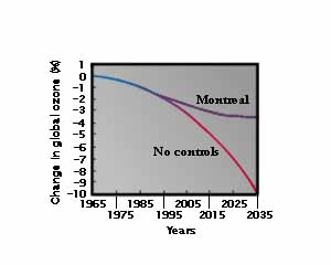
Theoretical models have been developed to predict future changes in ozone abundance. Figure 2 shows the results of one such projection into the future.

The Montreal Protocol was signed in 1987 and has since been strengthened. It commits to phase out production of the CFC's (first invented in 1930) by the turn of the century.

Without the Montreal Protocol, we would be looking at a disastrous reduction in ozone levels.

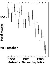
The Antarctic Ozone Hole

Figure 3.

The famous Antarctic Ozone Hole was discovered by British scientists who made systematic obseravtions of ozone using a simple ground instrument - the Dobson Meter. They published this famous figure that illustrated the downward trend of total ozone over Halley Bay, Antarctica in the month of October (austral Spring)..

These measurements of Farman et al., provided a wake-up call to the atmospheric science community. They were quickly verified by satellite observations and several campaigns were organized to find out what was happening in this region and during this particular time of the year.

The Farman et al., paper, published in 1985 showed a dramatic decrease in ozone. The decline from year to year has continued, more-or-less to this day.

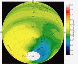
The figure shown below (figure 4) illustrate the satellite view of the same phenomena for the years leading up to the present. There are now several satellite missions that are dedicated to unraveling the chemistry and dynamics of ozone. These include the Total Ozone Mapping Satellite, TOMS and the Upper Atmosphere Research Satellite, UARS.

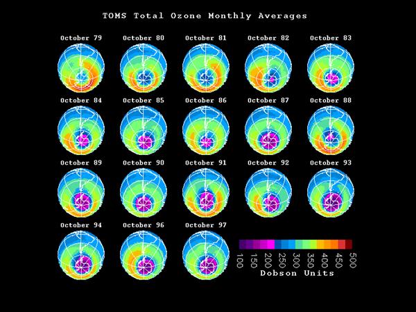
Figure 4.

The hole deepens and becomes enlarged from year to year, as well as deeper although not monotonically.

The Antarctic Ozone Hole is now well understood. Briefly what happens can be summarized as follows:

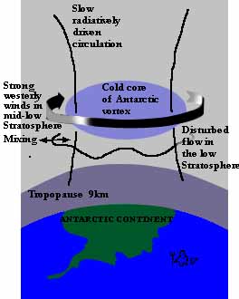
Figure 5.

The Antarctic Ozone hole is limited in space and time, occurring at the time of year when the Sun first appears above the horizon after the long polar night. During Polar Winter, a polar vortex forms and the polar air mass in the stratosphere becomes separated from other air masses. The temperature drops and drops, ultimately leading to the stratospheric air trapped in the vortex becoming very cold - in fact the coldest air to be found in any part of the Earth's stratosphere. In this cold vortex, polar stratospheric ice crystal clouds form. Gas phase HCl dissolves in the surfaces or clings to the surfaces of the clouds. The CFC's react with the HCl ice, converting relatively unreactive chlorine to the more active species, Cl2, ClONO2, and HOCl. At sunrise, in October, the chlorine-bearing compounds are photolyzed, releasing the highly reactive Cl atoms that attack ozone. Ozone densities drop rapidly, only to recover when the polar vortex breaks up, mixing warmer air in and releasing the ozone-depleted air to move away from the polar region. The ozone loss is felt globally!

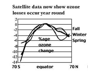
Northern Hemisphere Ozone

The Northern hemisphere is not immune from Ozone Holes. In the north, the stratospheric polar vortex is not as well formed as in the south. This is because of the larger contrast between land and water in the northern hemisphere. The existence of land masses tends to break up the symmetry of the polar vortex in the north. However, the same processes operate as in the south and satellite data show the effect occurring in March (Springtime in the northern hemisphere).

Sooner or later, we will see colder than usual northern polar stratospheric temperatures in the early Spring and heavily populated areas will be warned of unusually low ozone levels. Since ozone depleting compounds will be in the atmosphere for many tens of years, we have to live with these effects. Ultimately, chlorine compounds will cleanse themselves from the stratosphere and the Earth's ozone shield will return to normal - for our grandchildren's children.

For a movie showing the latest in Northern Hemisphere ozone hole formation, click here. For a movie showing the 1997 hole formation, click here

Potential Effects of Depleted Ozone

Of primary concern are the enhanced levels of UV radiation that reach the Earth's surface for a depletion in stratospheric ozone. It is customary to break up the UV spectrum into two parts:

UV-A: 400 - 320 nm
UV-B: 320 - 290 nm

The more energetic UV-B portion of the spectrum is responsible for sunburn, cataracts, potential ecological damage, and skin cancer. It can be absorbed by glass as well as by sunscreens and hats.

Relatively little is known or understood about the consequences of enhanced UV-B levels. We do know, however, that a 1% decrease in ozone abundance causes a ~2% increase in UV-B. Increased UV-B exposure at the Earth’s surface can impact human, agriculture and forest growth, marine ecosystems, biogeochemical cycles, and materials. Table 1 summarizes some of the potential effects of UV-B increases.

Table 1. Potential Effects of UV-B Increases.

Effects	State of Knowledge	Potential Global Impact
Plant Life	Low	High
Aquatic Life	Low	High
Skin Cancer	Moderate to High	Moderate
Immune System	Low	High
Cataracts	Moderate	Low
Climate Impacts^*	Moderate	Moderate
Tropospheric Ozone	Moderate	Low^**

^* Contribution of both stratospheric ozone depletion itself and gases causing such depletion to climate changes.

^**Impact could be high in selected areas typified by local or regional scale surface-level ozone pollution problems.

Effects on Human Health

Our best understanding of potential effects is in the area of skin cancers, for which detailed epidemiological records and studies exist. It is known, for example, that more than 90% of non-melanoma skin cancers are related to UV-B exposure. A 2% increase in UV-B is linked with a 2-5% increase in basal-cell cancer cases and a 4-10% increase in squamous-cell cancer cases.

In 1990, there were ~500,000 cases of basal-cell cancer in the U.S. and ~100,000 cases of squamous-cell cancer. A 1% depletion of ozone would cause an increase in skin cancer cases of ~20,000 per year. To put this rather alarming figure in context, it is necessary to discuss briefly the geographical prevalence of skin cancer in the U.S.

Figure 6.

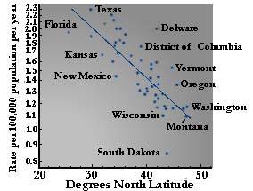
Figure 6 illustrates the rate of skin cancer as a function of latitude. While the data has some scatter, the trend is clear. A decrease of ~110 in latitude results in an increase of a factor of 2 in skin cancer occurrence. This occurs because the UV-B exposure increases towards the equator (~ a factor of 50 from pole to equator). An increase of ozone of 1% gives an increase of ~20,000 cases of skin cancer per year. This is equivalent to a southward shift in the average latitude of the U.S. population by only ~12 miles.

Actual ozone depletions at the latitude of the U.S. are ~1-3% already - primarily caused by chlorine catalytic chemistry. Figure 7 illustrates the global ozone reductions estimated from satellite data as a function of latitude and season. The depletions occur at all latitudes and seasons, but are most dramatic in the southern polar region in austral springtime (October). This depletion is the famous Antarctic Ozone Hole, as discussed above. We can see from this figure that we live in an ozone depleted world already. People living in the southern hemisphere are already well aware of this. Children growing up in Teirra del Fuego and New Zealand are very conscious of the need to wear hats in the midday sun. Daily news reports quote the ozone levels so that people can adjust their exposure to sunlight accordingly.

Figure 7.

Effects on Plants

UVB radiation affects plant physiological and developmental processes and can affect plant growth. Indirect changes, such as in the manner in which nutrients are distributed within the plan, the timing of developmental phases and secondary metabolism and plant form, may be as or more important than the directly damaging effects of UVB.

Effects on Marine Ecosystems

Phytoplankton are the foundation of aquatic food webs, and their productivity is limited to the upper layer of the water column in which there is sufficient sunlight to support net productivity. Exposure to solar UVB radiation affects phytoplankton orientation mechanisms and motility and lowers survival rates for these organisms. UVB radiation has also been found to damage early developmental stages of fish, shrimp, crab, amphibians and other animals.

Effects on Biogeochemical Cycles

Increases in solar UV radiation might affect terrestrial and aquatic biogeochemical cycles, which could affect sources and sinks of greenhouse and a number of other trace gases e.g., carbon dioxide (CO2), carbon monoxide (CO), carbonyl sulfide (COS) and possibly ozone. Such changes would contribute to interactions between the atmosphere and biosphere that attenuate or reinforce the atmospheric buildup of these gases.

Effects on Materials

Although a number of materials are now somewhat protected from UVB by special additives, synthetic polymers, naturally occurring biopolymers, and other materials of commercial interest are adversely affected by solar UV radiation. Increases in solar UVB levels will therefore accelerate their breakdown and limit their useful life outdoors.

Mitigation Strategies

Following the publication of the Farman et al. Findings in 1985, a series of ground-based and airborne measurements campaigns were conducted to develop an understanding of the chemistry and dynamics associated with the Antarctic Ozone Hole. This understanding lead to the Montreal Protocol on Substances that Deplete the Ozone Layer in October 1987. It required a freeze on the annual use of CFCs as early as 1990 with decreases leading to a 50% reduction by the year 2000. In 1990, the Montreal Protocol was amended to take into account the severe losses during the ozone hole events and the downward trends in global ozone. The participating countries substantially strengthened the protocol, calling for accelerated reductions in emissions, and requiring complete phase out of CFCs and other major ozone-depleting substances by 2000. The Montreal Protocol was further amended in 1992, calling for the complete phase out of CFCs, etc, by 1996.

Of Note

In 1996, Molina, Rowland and Crutzen received the first Nobel Prize (for Chemistry) to ever be awarded in Atmospheric Sciences. These scientists were instrumental in predicting the problem and in developing the needed scientific case for governmental action.

The 1995 Nobel Prize in Chemistry

Drs. Paul Crutzen, Mario Molina, and F. Sherwood Rowland were awarded the 1995 Nobel Prizes in Chemistry for their research on the science and implications of stratospheric ozone loss. The wording of their award is as follows:
"Paul Crutzen, Mario Molina and Sherwood (Sherry) Rowland have all made pioneering contributions to explaining how ozone is formed and decomposes through chemical processes in the atmosphere. Most importantly, they have in this way showed how sensitive the ozone layer is to the influence of anthropogenic emissions of certain compounds. The thin ozone layer has proved to be an Achilles heel that may be seriously injured by apparently moderate changes in the composition of the atmosphere. By explaining the chemical mechanisms that affect the thickness of the ozone layer the three researchers have contributed to our salvation from a global environmental problem that could have catastrophic consequences."

The Blue Planet

1. Composition and Salinity of the Oceans

Planet Earth has been called the "Blue Planet" due to the abundant water on its surface. Here on Earth, we take liquid water for granted; after all, our bodies are mostly made of water. However, liquid water is a rare commodity in our solar system. There is no liquid water on the Sun nor anywhere else in the solar system, save Earth. Nor has a drop of water been observed in interstellar space. Only a planet of the right mass, chemical composition, and location can support liquid water. Only on such planets could life flourish.

Liquid water covers most of the surface of our planet. This water comes in many forms, each with it's own special properties. Rain is essentially pure water (consisting only of H₂O), while spring water contains dissolved salts (~0.02-0.4%). Ocean water is the saltiest, with several ppm dissolved salts. The word "brine" is used to describe water that is saturated with salts. These different types of water are found in different environments on Earth.

The largest and most dramatic bodies of water are our oceans. The oceans cover ~71% of the globe and have an average depth of 3,729 meters. They have an average salinity (amount of dissolved salt) of 3.47% or 34.72 parts per mill (ppm). Seawater also contains lots of solutes in addition to salt. The mean residence times for ions that are involved in biological cycles (e.g. bicarbonate HCO₃-) are shorter than those for ions that are created by primary production and lost by undersea volcanism and wet subduction (e.g., Na+, Cl-).

The oceans are extremely important in regulating climate. Over half of the solar radiation absorbed by our planet is taken up by the oceans. This energy, once absorbed, is redistributed by ocean currents. The mass movement of water performed by the oceans plays a key role in the control of climate.

Temperature and Salinity

Figure 1. The salinities of Earth's Oceans measured in ppm

An important attribute of liquid water is its ability to hold dissolved ions in solution. The density of water increases as its salinity increases. This has profound effects on ocean circulation and nutrient transfer rates.

When water evaporates, it leaves behind dissolved salts, making the remaining water more dense and likely to sink to the ocean floor. In this way important nutrients (such as dissolved oxygen) are cycled to the ocean floor in a process known as "bottom-water formation". Also, the sinking action of saline water can drive large-scale ocean circulation (see below). Subsurface ocean circulation produced by a combination of temperature and salinity is called "thermohaline circulation". This type of circulation is distinguished from the surface circulation, which is wind-driven.

Figure 2: Thermal structure of Earth's Oceans

The salinities of the Atlantic and Pacific oceans are shown in Figure 1 for north-south cross-sections of the Atlantic and Pacific oceans. Note the effect of enhanced salinity due to outflow from the Mediterranean.

The North-South thermal structures of the Atlantic, Pacific, and Indian oceans are shown in Figure 2. Several features are of interest in this figure. Temperature tends to maximize at the surface, with the deep waters being largely isothermal (having a constant temperature with depth). As a consequence, the temperatures are high in the top 1000 meters and drop thereafter. The warmest temperatures are near the equator, as expected, with the polar water being relatively cold and isothermal. Because of the nature of the thermal structure, it is often useful to think of two separate ocean reservoirs

2. Ocean Circulation

Unlike the atmosphere, which is characterized by turbulent weather systems, the ocean is a fairly stable place. This is because it is heated from above, in contrast to the atmosphere, which is heated from below.

Warm water is less dense (heavy) than cold water. The relatively warm surface waters, therefore, tend to remain floating on top of the colder and denser deeper waters. This tendency leads to a generally stable situation which inhibits turbulence. If the deep ocean were never to move, however, we would find no oxygen and no aerobic life at deep levels. Since life is plentiful there, it is evident that some large-scale motion occurs in the oceans, allowing deep waters to become oxygenated.

The ocean has four types of motion:

· surface currents

· deep circulation

· tides

· tsunamis

Different sources provide energy for these different types of motion. Surface and deep currents are powered by solar radiation. The energy source for the tides is gravitational attraction of the Earth and Moon. The Earth's internal heat provides energy for tsunamis. We will focus on the first two types of circulation: surface currents and deep currents.

Figure 3. Global Surface Currents.

Large-Scale Surface Currents

Surface currents are forced by frictional interaction between the ocean surface and the prevailing atmospheric wind. The wind imparts its momentum to the top layer of the ocean.

In each ocean, the prevailing trade winds drive equatorial ocean currents from east to west. When these currents encounter land, they divide to flow north and south along the eastern borders of the continents. As they progress, they are deflected to the right in the Northern Hemisphere and to the left in the Southern Hemisphere by the Coriolis Effect (see climate patterns lecture), creating large vortices or gyres.

Figure 3 illustrates the large-scale surface currents. Notice the large clockwise gyres in the Northern Hemisphere and the counter-clockwise gyres in the Southern Hemisphere. Small west-to-east counter-currents are seen near the equator. The famous Gulf Stream (currents number 1 and 2) carries more than 20 times the total amount of water in all the rivers and streams in the world!

Smaller-Scale Surface Currents:

The Coriolis Effect forces surface water at an angle of ~45^o to the direction of the wind. As momentum passes downwards through ocean layers, the currents rotate further under the influence of Coriolis and moderate. The net result is what is known as an "Ekman Spiral" motion (shown in Figure 4). On average, the surface waters, taken as a whole, tend to move perpindicular to the prevailing wind (to the right in the Northern Hemisphere and to the left in the Southern Hemisphere).

Figure 4: Ekman Spiral for Northern Hemisphere

· Figure 4 shows the Ekman Spiral for the Northern Hemisphere. For a wind blowing southward along the coast of California, the ocean current will be seaward.

· The region over which the current actually reverses direction is known as the friction layer (~100 m depth).

· The Ekman Spiral helps explain why the waters off the coast of California are so cold (see Figure 5).

· The cold waters off the coast of California are clearly unusual. Water temperatures closer to what one might expect for the latitude (about 10^°F higher) are found to the north and the south of the localized cold zone.

The Ekman Spiral has a different direction in the Southern Hemisphere than in the Northern Hemisphere, where the rotation is towards the right.

Figure 5. Ocean temperature isoclines off the West Coast of North America.

The cold waters off California are produced by the same process that results in cold surface waters off the western coasts of South America and Africa. The process is related to the offshore surface current driven by the prevailing winds, which blow parallel to the coast.

Figure 6. Upwelling off the California Coast.

Figure 6 shows the geometry for the case of California surface waters. The prevailing wind blows from north to south along the coastline and, in conjunction with the Coriolis Effect, forces the surface waters west and out to sea. The waters in this seaward current are replaced from below. The forced upwelling of cold deep water cools the surface waters and brings vital nutrients upwards to support a rich food chain, including large numbers of photosynthetic phytoplankton. This situation in Californian coastal waters is repeated off the coast of Peru, with the difference that the Peruvian cold waters are in the Southern Hemisphere. The Peruvian waters support an incredibly rich food chain, including the world's most important anchovy fishery.

El Niño

Since the upwelling currents are forced by prevailing winds, they are affected by changes in the strength of these winds. A phenomenon known as El Niño occurs periodically in Peruvian coastal waters. This term refers to the occasional situation when the trade winds slacken sufficiently to cut off the Peruvian upwelling, leading to an increase in the temperature of the surface waters. It is called El Niño (the Christ-Child in Spanish), since it often occurs around Christmas time. During these events, most of the photosynthesizing (phytoplanktic) sea creatures are starved of the nutrients normally brought up from the deep waters and die away. Sometimes, the die-off is so rapid and intense that the decomposing bodies of the sea creatures leave a foul smell on the ocean.

Figure 7. El Niño influence in the Pacific Ocean.

Figure 7 shows the region of the Pacific Ocean that is anomalously warmed during El Niño events. The size and extent of surface-water warming affects the Earth's climate on a truly global scale, with certain areas of the world experiencing drought while others experience greater rainfall.

El Niño events occur sporadically every 3-5 years or so and last for a year or two. Some of the unusual weather we experienced in 1997-98 has been ascribed to an El Niño event. A new and interesting theory attempts to correlate El Niño events with equatorial volcanic eruptions (which would affect the strength of the trade winds).

· El Niño events are also sometimes referred to as "ENSO" events (standing for El Niño, Southern Oscillation events). One of the effects of an ENSO event is a rise in sea level off the coast of South America and a drop in sea level off Australia.

· El Niño events occur sporadically but fairly often (one every 3-5 years or so). They are almost impossible to predict.

· The opposite (and more normal) situation to El Niño is sometimes called "La Niña" - good fishing time!

Deep Water Circulation - The Thermohaline Circulation

Figure 8. Great Ocean Conveyer Belt.

A large-scale circulation of the oceans involving a deep current carries more than 30 times the volume of all the rivers of the world combined. We will call this 3-dimensional current the "Conveyor" (Figure 8).

The conveyor belt is a globe-straddling ocean current that keeps Northern Europe unusually warm for its latitude. The Gulf Stream is one leg of this current system. It functions to transfer heat from the relatively warm tropics to the relatively cold polar regions.

The extra heat received by Northern Europe is brought by the conveyor-belt-like ocean current. The part of the conveyor near the ocean surface moves to the North in the Atlantic and to the south in the Pacific. In the Atlantic, the surface of the conveyor carries warm water to a region near Iceland, where it cools and sinks, returning at great depth. The convergence of warm surface current and cold Arctic air allows for effective transfer of heat to the atmosphere, keeping Europe warm. The amount of heat involved is very large: about 30% of the total solar energy received by the entire Atlantic! As the waters cool due to this heat transfer conveyor, they become more dense and sink, feeding the lower part of the conveyor.

The sinking action of the conveyor at its northernmost extreme in the Atlantic is aided by its extra salinity. There is a slight imbalance between evaporation and runoff in the Atlantic, which causes it to be saltier than the Pacific. (Some of the water evaporated from the Atlantic ends up precipitating into the Pacific, either directly or from runoff via rivers and streams. Water evaporates in its pure form, leaving behind salt and other solutes. The net effect of this imbalance is to make the Atlantic more saline than the Pacific.) This difference in salinity between the Atlantic and the Pacific is a driving force behind the Conveyor. This type of circulation, powered by differences in temperature and salinity, is referred to as Thermohaline Circulation (Heat-Salt Circulation).

Figure 9. Energy transfer through the Conveyer Belt.

The importance of the conveyor to climate is impossible to overstate. Without its moderating influence on the climate of Europe, Paris would have roughly the same climate as the Hudson Bay and human history would have been quite different! Figure 9 illustrates the effect of the transfer of energy from the warm surface current to the air blowing from Canada towards Europe.

To recap: at the northern Atlantic limit of the ocean conveyor belt, surface waters release heat into the atmosphere, greatly moderating Europe's climate. The subsequent plummeting of the cooled water to greater depths simultaneously enriches the bottom waters with oxygen, allowing life in the deep ocean. The cycle is powered, in part, by the extra salinity of the Northern Atlantic waters, due to the higher rate of evaporation compared to the Pacific.

There is evidence that the conveyor has stalled once within the past 10,000 years during the brief cooling period known as the Younger Dryas.

3. An Example of Rapid Climate Change Caused by Air-Sea Interactions: The Younger Dryas

The Younger Dryas was a period of dramatic cooling that occurred during the warming trend to the current interglacial - ~10,000 years ago. The Younger Dryas period lasted ~700 years and led to enormous but short-lived changes in the climate of Northern Europe. These changes were first noted in the pollen records, which indicate a change-over from forests to herbaceous plants (such as Dryas, a plant that thrives on glacial tundras) and back to forest again. In the early 1980's, evidence for the Younger Dryas was obtained from CO₂ ice-core bubble measurements also, confirming that it was an event of global significance (since carbon dioxide is well-mixed throughout the global atmosphere).

The Younger Dryas period has caused much debate, since it challenged the previously-held idea that climate could only change very gradually. It had been thought that the thermal inertia of the ice sheets was so large that significant advances or retreats could only happen over long periods of time. The Younger Dryas demonstrated unambiguously that change can be abrupt. Climate appears sometimes to respond in a manner similar to earthquakes where stress and strain builds up over years, leading to sudden abrupt changes, rather than slow incremental changes.

Figure 10 provides a synopsis of what we suppose happened to the temperature of the North Atlantic Basin during the Younger Dryas. The top panel shows the changes in solar radiation expected from a consideration of the Milankovitch cycles over the past 30,000 years. The bottom panel shows the sluggish (lagging) response of the melting ice caps. The middle panel shows the paleoclimate temperature record.

Figure 10. Conditions leading up to and
during the Younger Dryas.

Figure 11. Retreat of the polar ice cap.

Consider the melting of the polar ice cap as it retreated (Figure 11). Initially, all the runoff waters would have been channeled into the Gulf of Mexico along the Mississippi and its tributaries. At some point, when the glaciers had retreated to about the latitude of Northern Lake Superior, the runoff waters would have been diverted to flow out along the St. Lawrence into the Northern Atlantic. Since these fresh waters had very low salinity, they would have inhibited the downward plunge of the conveyor belt off the coast of Labrador. This sudden release of vast amounts of fresh water into the Northern Atlantic might have been sufficient to stall the Conveyor belt completely, leaving Europe without its moderating influence. After the initial shock of the fresh water runoff had been absorbed, the Conveyor would have started up again, returning the climate to its ordained "Milankovitch cycle" path. The timing of the retreat of the polar cap ice past Lake Superior has been shown to be coincident with the onset of the Younger Dryas, within errors.

The example of the Younger Dryas is a warning that climate change can be unpredictable and abrupt. Stresses on the system can build up until, almost without warning, a sudden and fundamental change occurs on a short time scale.

Summary

1. The oceans play an important role in controlling the climate of the Earth. Both temperature and salinity contribute to the establishment of the 3-dimensional thermohaline currents that encircle the globe.

2. The ocean is fundamentally stable since it is heated from above. The temperature structure defines a shallow warm surface region (~5% of the total) and a deeper cold layer (~95% of the total).

3. Surface water gyres and the Conveyor Belt both effectively transport energy from low to high latitudes. The Conveyor moderates the climate of Northern Europe.

4. Upwelling of cold, nutrient-rich waters on the west coasts of continents is forced by a combination of prevailing winds and the Coriolis Effect. When upwelling off the coast of Peru occurs, we have the El Niño condition, which can cause global climate changes.