Unit 8a. Analysis of Vostok Ice Core Data
 Objective
One of the primary results of paleoclimate
research over the past decade has been strong evidence for human-influenced
(anthropogenic) global warming. Results have been based on ice cores taken from
undisturbed ice sheets, such as those in
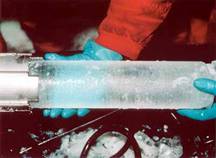
Figure 8.a.1
Ice core
Vostok is the Antarctic research
base founded by the
Subglacial 
Figure 8.a.2
Antarctica with
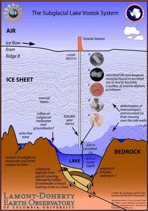
Figure 8.a.3
The subglacial
Part 1. Ice and Gas Ages in the Vostok Core
Open the excel file entitled vostokdata.xls. Click on the Vostok tab of the excel sheet. This dataset contains columns that give the depth (in meters) of the ice core, the "ice" and "gas" ages (in thousands of years ago), concentrations of carbon dioxide and methane found in the ice bubbles, the hydrogen isotopic ratios, and a column that provides information on dust.
The ice age (i.e., the age of the ice, not to be confused with our other use of the term ice age, which refers to a time in geologic history of pronounced glaciation) is obtained by counting layers of ice and, when layers are no longer clearly visible, modeling the flow of merged ice layers.
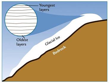
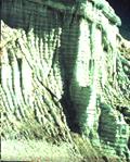
Figure 8.a.4
Annual ice layers
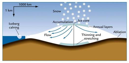
Figure 8.a.5
Continental ice sheets
The gas age is calculated assuming that the bubbles of gas can only be trapped effectively in layers of older ice (i.e., at a depth well below the surface, where the pores in the ice close, sealing the air). This process is called sintering.
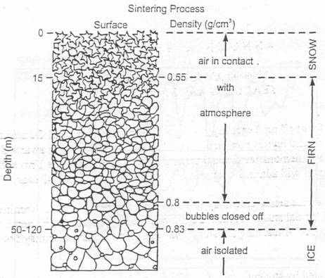
Figure 8.a.6
Sintering process - Raynaud, 1992
Plot both the ice age and the gas age as a function of
depth: first select the entire ice age column by clicking on the "B"
at the top of it, then hold down the control key, and then select the gas age
column by clicking on the "E" at the top. Once both are selected,
click on the "Chart Wizard" ![]() icon and select the first line graph (without
markers) option. Click “Next”. In step 2 of the chart wizard, modify the series
data (click on the series tab) to use the depth values in column A as the
category (X) labels. You will need to specify the numbers themselves, not the
whole column. The formula for the X values for both series should look like
this: =Vostok!$A$3:$A$196. Now click "Next,"
and give your chart appropriate labels for the title and axes. Be sure to label
the appropriate units. If you don't know what they should be, then re-read this
lab again from the beginning. You should always know what you are graphing and
why! Next, place the chart as an object in your Vostok
Data worksheet.
icon and select the first line graph (without
markers) option. Click “Next”. In step 2 of the chart wizard, modify the series
data (click on the series tab) to use the depth values in column A as the
category (X) labels. You will need to specify the numbers themselves, not the
whole column. The formula for the X values for both series should look like
this: =Vostok!$A$3:$A$196. Now click "Next,"
and give your chart appropriate labels for the title and axes. Be sure to label
the appropriate units. If you don't know what they should be, then re-read this
lab again from the beginning. You should always know what you are graphing and
why! Next, place the chart as an object in your Vostok
Data worksheet.
Question 8.a.1
The two age curves differ - why?
How much younger, roughly, is a bubble of gas than the ice that surrounds it,
at a depth of 1000 meters?
 Part 2. The Temperature Record
Oxygen has two stable isotopes of importance, 16O and 18O, which vary in mass. Differences in the amounts of these isotopes in an oxygen-bearing molecule are measured by using a ratio of 18O/16O and then that ratio is compared to the ratio of 18O/16O in average ocean water. This comparison is called d18O (pronounced delta-18-O). Variations in the d18O of the oxygen in the water molecule, H2O, can be useful in understanding the hydrological cycle. Average ocean water has a value of 0‰ d18O (‰ is pronounced permil and is the symbol for one-thousandth. It is analogous to %, percent, which is the symbol for one-hundredth).
Figure 8.a.6
Layers of ice
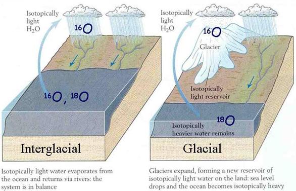
Figure 8.a.8
Isotopic signature during glacial and interglacial periods
When ocean water evaporates, water with the lighter oxygen isotope (16O) evaporates more easily because it is lighter than a water molecule with the heavier oxygen isotope (18O). Therefore, water vapor in the atmosphere ends up with a smaller percentage of 18O in it than ocean water. Its d18O is a few permil negative, say around –3‰. When that vapor passes over land and condenses to form rain, the heavier isotopes that did make it into the clouds condense to a greater extent than the lighter isotopes, again due to mass. Precipitation that falls then has a more negative d18O than seawater, but more positive d18O than the clouds from which it fell. This effect is more pronounced in cold climates than in warmer ones, because temperature is what drives the evaporation/condensation processes. Snow has much more negative d18O than rain. Since temperature drives this process, an equation has been derived to relate temperature to d18O.
Hydrogen isotopes of interest to paleoclimate studies are 1H and 2H. Since 2H is such an important isotope to nuclear chemistry, it has its own name: Deuterium.
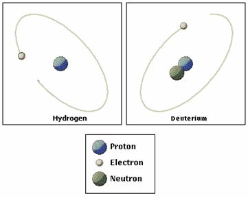
Figure 8.a.9
Structure of Deuterium
The scale we use here to describe the variation in hydrogen isotopic ratios of substances is dD (pronounced delta-D). For most precipitation on Earth, the following relationship applies: dD = 8 * d18O + 9.
We want to convert the deuterium isotopic ratios to temperature changes (delta temperatures) that describe variations in the temperature of the ocean from which the ice was originally evaporated. Type "delta temp" in the first row of your new column and "(deg C)" in the second row. Now use excel to calculate the delta temperatures, filling in your new column (use the Excel help menu if you do not know how to do this). Highlight the column and give the numbers two decimal places. Use the following relationship:
 Type
"= (N7 + 440) / 6.2" into the first cell, then put the cursor
on the lower right corner of the cell until it turns into a gray cross. Click
and hold the left mouse button and drag down to the end of the column. The
cross cursor applies the relationship of the first cell to other cells.
Type
"= (N7 + 440) / 6.2" into the first cell, then put the cursor
on the lower right corner of the cell until it turns into a gray cross. Click
and hold the left mouse button and drag down to the end of the column. The
cross cursor applies the relationship of the first cell to other cells.
Figure 8.a.10
Drilling ice cores at Vostok
Save your work. Think about why the delta temperatures change with deuterium isotope ratio in the way they do. If you don't understand, then you should be sure to read through the suggested readings listed at the end of this lab.
Question 8.a.2
Plot the delta temperature curve as a function of ice age (use either a line or scatter plot) and copy it into your report. How many degrees has climate varied in the past, as indicated in these data?
Question 8.a.3
Approximately when did the last
glacial period begin and end? When did the last interglacial time period begin
and end? Within the most recent glacial period, what were the highest and
lowest delta temperatures? What do you think your hometown might have looked
like at these times?
Part 3. The Atmospheric Composition and Dust Record
Use the following scatter plots of CO2 and CH4 concentration, as well as delta temperature and dust as a function of (ice) age, to answer the questions for this section. These were made from the same data you are using, and you may want to replicate them yourself to get more practice with Excel.
Figure 8.a.11
Carbon dioxide and methane concentrations plotted with delta temperature
Figure 8.a.12
Dust and temperature as a function of age
Question 8.a.4
Note the time of the two major warming events. Then look at how CO2 and CH4 change during the same time. From the data provided in this lab, can you tell which changes first, temperature or greenhouse gas (CO2, CH4) composition? (Note the direction of the x-axis.) Suggest reasons why it could work either way.
Question 8.a.5
These graphs do not show recent
values. What are several reasons why CO2, CH4, and dust
concentrations were different during the glacial and interglacial periods?
Predict how the Industrial Revolution might have affected the global
concentration of CO2, CH4 and dust.
Part 4. What can we learn from all this about climate today?
First add another column to your Excel file to estimate the temperature at Vostok. Label the column Vostok Temp. (deg C). To do this subtract 55.5 degrees from the numbers in the delta temperature column to get an estimate of the Vostok temperature itself.
Create scatter plots (without connecting lines) of CO2 (x-axis) vs. temperature (y-axis) and CH4 (x-axis) vs. temperature (y-axis) using the Vostok data. Use the Insert a linear "trend line" and report the equation and r2 value by checking those boxes in the option menu for trend lines of each scatter plot in your lab report. The r-squared (r2) is a statistical measure of how well a regression line approximates real data points; an r-squared of 1.0 (100%) indicates a perfect fit. So if you had an r2 of 1.0 for the CO2 vs. temperature plot, if you knew the CO2 concentration you could predict the corresponding temperature 100% of the time.
Question 8.a.6
Copy your scatter plots with trendlines into your report. Why is the r2 value for CO2 or CH4 less than one?
Question 8.a.7
Predict the temperature at Vostok today. Use today's CO2 concentration (385 ppmv) to solve the linear regression equation from the past relationship between CO2 and temperature. How does this calculated temperature differ from the surface temperature today at Vostok? Explain why these may be different. (you can look up this temperature with a weather website)
Extra Credit (Optional):
Click on the Insolation tab of the excel data sheet containing the Milankovitch cycle variations of solar insolation for the last million years (data from Berger, 1991). The first column represents thousands of years before the present (ka) and is given a negative number. The other columns represent the insolation in watts per meter squared at the specified dates and latitudes. Make a plot of the insolation curve over the period of the Vostok data record and compare it with the Vostok temperature plot.
Question 8.a.8
Can you see evidence of the Milankovitch cycles? Discuss the relationship - similarities and differences between the Vostok temperature plot and the solar insolation plot due to orbital changes. Can you find a way to merge these data sets?
Sources
Monnin et al. "Atmospheric CO2 concentrations over
the last glacial termination" Science v.291, 112-114, 5 January
2001.
Dansgaard, W., H.B. Clausen, N. Gundestrup,
C. U. Hammer, S. J. Johnsen, P. M. Kristinsdottir, and N. Reeh, A
New Greenland Deep Ice Core, Science, Vol. 218, 1992, p.1273-1277.
"Deciphering
Mysteries of Past Climate From Antarctic Ice Cores" Earth in
Space (American Geophysical
Crane,
Robert G., James F. Kasting, and Lee R. Kump. The Earth System.
http://www.aad.gov.au/asset/images/525_ul-core.jpg
A great source of paleoclimatological data can be found at the NOAA web site.