Unit 7a. Earth’s Energy Balance Model
Objective
The sun radiates energy outward toward the planets, which provides
light and heat to the Earth. At the same time, the Earth radiates energy back
into space. In this exercise, we will use STELLA to create a model showing
these energy flows and the equilibrium that is reached. This model is
relatively simple, yet very powerful: it describes the temperature of our
planet, one of the key factors that have led to the evolution of life.
Figure 7.a.1
The sun
Part 1. Define the Problem and Goals of the Model.
The primary goals of this exercise are to illustrate the physical processes that dictate the Earth’s temperature, and to create a model that accurately predicts the radiative equilibrium temperature that maintained the early Earth’s energy balance. It is important that you understand the basic assumptions and conclusions of the model to understand how this process works as a system, so that you can incorporate information learned later on and build on your modeling skills.
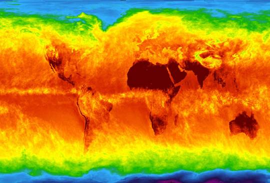
Figure 7.a.2
Picture of the IR radiation of Earth
Part 2. Understand the Real Life System.
Let’s first consider the stocks and flows that will comprise the heart of our model. The thing that accumulates in our system is energy. So we will represent Earth energy as a stock in our model. The processes affecting this stock are (1) Earth’s capture of solar radiation; and (2) the emission of infrared energy from Earth to space. We will represent these processes by flows into (solar to Earth) and out of (Earth to space) the Earth energy stock (Figure 7.a.3).
Figure 7.a.3
Initial components of the Earth energy balance model
Figure 7.a.4
Solar to Earth
Next, identify the radiation laws and other physical properties that govern these flows. We know that the amount of solar radiation reaching the Earth (or any other planet) is a function of its diameter, albedo (ability to reflect radiative energy), and distance from the sun (solar constant as predicted by the "R-squared Law").
So in our model we will have three converters feeding into the solar to Earth flow: solar constant, Earth albedo and Earth diameter (Figure 7.a.4). (Note: diameter is twice the radius)
The equation governing this relationship is:
Equation 7.a.1.
solar to Earth = solar constant * (1 – Earth albedo) * PI * (Earth diameter / 2) ^2
Similarly, the Stefan-Boltzmann law tells us that the amount of energy emitted by an object goes as the fourth power of its temperature ("E equals sigma T to the fourth"). Therefore, the amount of radiative energy lost from the Earth can be calculated as follows:
Equation 7.a.2.
Earth to space = PI * (Earth diameter^2) * sigma * Earth temperature^4
Thus our model will contain three converters feeding into the Earth to space flow: Earth diameter, sigma, and Earth temperature, where sigma represents the constant in the Stefan-Boltzmann equation (Figure 7.a.5).
Figure 7.a.5
Earth to space
Finally, the first law of thermodynamics tells us that a body’s temperature is given by its energy divided by its heat capacity:
Equation 7.a.3
Earth temperature = Earth energy / heat capacity
And, given that the surface of the "blue planet" is primarily comprised of water, we can use the properties of water to calculate the Earth’s heat capacity (by making the simplifying assumption that the Earth is covered by a uniform layer of water.)
Equation 7.a.4
heat capacity = PI * (Earth diameter^2) * water depth * density of water * specific heat of water
So our final model should look equivalent Figure 7.a.6 below (do not try to simply copy Figure 4, it will not work, go through the directions step by step):
Figure 7.a.6
Complete model structure
Part 3. Build the Model.
1. Start up STELLA.
2. To get into modeling mode, click once on the globe icon on the left hand side of your screen, so that it changes to a X2 (Chi-square) symbol. You are now ready to start modeling. Note: in this model, all units are written out within "curly" brackets: {}. The units entered inside the curly brackets are notes that are not read by STELLA but allow you to keep track of your units. You may also use the units button to enter them, or simply type the units out exactly as they are in the lab, including the brackets.
3. Create the Earth energy
stock by clicking on the stock icon ![]() and then on the screen. To name the stock: type Earth energy in to the highlighted text area. Then double-click on
the question mark to set the initial value. Type 0.00 in the dialog box and click OK. This allows us to watch the
Earth warm up from its initial temperature of absolute zero.
and then on the screen. To name the stock: type Earth energy in to the highlighted text area. Then double-click on
the question mark to set the initial value. Type 0.00 in the dialog box and click OK. This allows us to watch the
Earth warm up from its initial temperature of absolute zero.
4. Create a flow into the Earth energy stock. (Click on the flow icon ![]() ,
place the pointer to the left of Earth
energy, and by dragging the
mouse, join the flow to the stock. Make sure there is only one
"cloud" attached to the flow icon.) Name the flow solar to Earth.
,
place the pointer to the left of Earth
energy, and by dragging the
mouse, join the flow to the stock. Make sure there is only one
"cloud" attached to the flow icon.) Name the flow solar to Earth.
5. Now create another flow out of the Earth energy stock and name it Earth to space. (Click on the flow icon, place the pointer inside the stock and drag the mouse outside of the box. Again, make sure there is only one "cloud" attached to the flow icon.) At this point your model should look like Figure 7.a.3.
6. We will now add a number of converters to the model, each of which will contain one of the constants needed for our stimulation.
7. Click on the converter
icon ![]() ,
place it near the solar to Earth,
and name this first converter solar
constant. Double-click on the question mark, type in 1368 {J/(m^2 * s)} * 3.15576E7 {seconds per
year} as the value, and click OK. (3.15576E7 is used to express 3.15576
x 107, the scientific notation for 31, 557, 600.
,
place it near the solar to Earth,
and name this first converter solar
constant. Double-click on the question mark, type in 1368 {J/(m^2 * s)} * 3.15576E7 {seconds per
year} as the value, and click OK. (3.15576E7 is used to express 3.15576
x 107, the scientific notation for 31, 557, 600.
8. Repeat step 7 to create two more converters named Earth albedo and Earth diameter. (Hold down the option key to retain the last building block, tool or object you used.) Define the values of Earth albedo and Earth diameter to be 0.30 and 12742E3 {m} respectively.
9. Now connect the converters, one by one, to solar Earth using connectors. Do this
by clicking on the connector
icon ![]() ,
placing the pointer on the boundary of the converter and connecting it to solar to Earth. The left side of your
model should look like Figure 2.
,
placing the pointer on the boundary of the converter and connecting it to solar to Earth. The left side of your
model should look like Figure 2.
10. Repeat step 6 to add a converter below the Earth to space flow called sigma (Stefan-Boltzmann constant). Once again use the connector tool to connect sigma to Earth to space, and set the value of this constant equal to 5.67E-8 {J/(m^2 * s * K^4)} * 3.15576E7 {seconds per year}.
11. To add a second Earth
diameter converter near Earth to
space, we will need to use a ghost
icon ![]() to indicate that it is the same constant used
on the left side of the model. Ghost icons are used primarily for aesthetic
purposes, to improve the legibility and comprehensibility of a model (avoiding
the "spaghetti" that accumulates when there are too many connectors
criss-crossing each other).
to indicate that it is the same constant used
on the left side of the model. Ghost icons are used primarily for aesthetic
purposes, to improve the legibility and comprehensibility of a model (avoiding
the "spaghetti" that accumulates when there are too many connectors
criss-crossing each other).
Click on the ghost
icon ![]() ,
and then on the original Earth diameter
converter. Then click near Earth to space to add another copy of this converter
to the model. (The ghost converter should look shadowy, with a dotted outline.)
Connect it to Earth to space.
The value of this converter should already be set.
,
and then on the original Earth diameter
converter. Then click near Earth to space to add another copy of this converter
to the model. (The ghost converter should look shadowy, with a dotted outline.)
Connect it to Earth to space.
The value of this converter should already be set.
12. Create another converter named Earth temperature below the Earth energy stock to represent the radiation equilibrium temperature of the planet. Insert one connector from Earth temperature to Earth to space, and another from Earth energy to Earth temperature (since temperature depends on energy)
13. Before we can define Earth temperature, we must add heat capacity to the model. Create another converter below Earth temperature and name it heat capacity. Insert a connector from heat capacity to Earth temperature.
14. Now we will add the converters that are needed to define heat capacity. Add three more converters named water depth, specific heat of water and density of water, and connect them one by one to heat capacity. Set the values of these constants to 1.0 {m}, 4218 {J/(kg * K)} and 1000 {kg/m^3}, respectively.
15. Finally, repeat step 11 to add another ghost converter for Earth diameter and then connect it to heat capacity.
16. Now we are ready to input equations. Double-click on the heat capacity icon and use Equation 7.a.4 to define the value of this converter:
PI*(Earth_diameter^2)*water_depth*density_of_water* specific_heat_of _water.
PI can be found in the "builtins" list on the right side of the dialog box. (Make sure to use the list of required inputs to enter variable names, rather than typing them manually. STELLA will not accept variable names that do not match exactly.)
17. Repeat step 16 for the Earth temperature converter, using Equation 7.a.3. Then use Equations 7.a.1 and 7.a.2 to define the solar to Earth and Earth to space flows, respectively.
All done! Your model should now look like Figure 7.a.6.
Part 4. Test the
Model.
Now run the model with initial Earth energy of zero. We are interested in observing the change over time in Earth energy, Earth temperature and Earth to space.
Insert a numeric
display box on your workspace above your model using the ![]() icon. This will allow you to see the numeric
value of a certain variable at the end of the simulation. Double-click on your
empty numeric display box and select Earth temperature. Make sure "retain
ending value" is selected, and leave other options at the default
settings.
icon. This will allow you to see the numeric
value of a certain variable at the end of the simulation. Double-click on your
empty numeric display box and select Earth temperature. Make sure "retain
ending value" is selected, and leave other options at the default
settings.
To view the model output, click on the graph icon ![]() and then click on the screen to bring up a graph window, which will not yet
have a legend on the y-axis. Double-click on the graph to select which
variables to show. Select Earth energy,
Earth temperature, and Earth to space by highlighting them in
the allowable column and then
moving them to the selected
column by clicking on >>. In the space for the title, enter "Earth
Energy Balance." Click OK to close the dialog box.
and then click on the screen to bring up a graph window, which will not yet
have a legend on the y-axis. Double-click on the graph to select which
variables to show. Select Earth energy,
Earth temperature, and Earth to space by highlighting them in
the allowable column and then
moving them to the selected
column by clicking on >>. In the space for the title, enter "Earth
Energy Balance." Click OK to close the dialog box.
To run and plot the graph, select run specs from the run menu. In the dialog box that appears, input the length of the simulation (from 0 to 1.00), time step (DT = .01) and unit of time (years). These parameters mean that we are modeling the change in the Earth’s energy balance over a period of one year, in increments of 1/100 year. Click OK to return. Select run from the run menu on top of the screen to execute the model.
Figure 7.a.6
Graph of Earth’s energy, Earth’s temperature and Earth to space radiation
Looking at the output graph, we see that the model in the equilibrium region predicts a radiative equilibrium temperature of 255 K (-18C). This is the temperature that results in a balance between radiation received by the sun and infrared emissions from the Earth.
You will also notice that the curves for Earth energy (1) and Earth temperature (2) have the same shape. This happens here because the two variables are in direct proportion to one another (although the actual values are different, as illustrated by the scales shown along the Y-axis). The Earth to space (3) curve has a different shape because it is proportional to the fourth power of Earth temperature (T4). When T is small, relative to its maximum value, the T4 is very, very small as shown on the lower left corner of the graph; as the two variables approach their maximum values, Earth to space catches up with Earth temperature and they both attain their equilibrium values. (The Y-axis scales for Earth energy and Earth to space show zeros trailing of the chart because STELLA is trying to display all the variables in the same numerical units (i.e. not scientific notation).
|
Units |
|
|
J = Joule |
s = second |
|
m = meter |
yr = year |
|
K = degrees Kelvin |
kg = kilogram |
Table 7.a.1
Model units and abbreviations
Explore the Model
Question 7.a.1
List three model assumptions that are made in the above model. Explain each assumption.
Save your Earth model, then save a second copy as "Venus model". Adjust your Venus model to predict the temperature of Venus. We will assume the same heat capacity as in the Earth model, and use the Venus diameter and distance from the sun shown in Table 7.a.2. There are two other inputs that need to be modified: Venus albedo and solar constant.
Remember that the value for the solar constant that we used in the Earth model was adjusted for the Earth’s distance from the sun. We can re-adjust this for Venus’ distance from the sun by multiplying the value we used by R2E/R2V, which is the ratio of Earth’s distance from the sun squared to Venus’ distance from the sun squared (refer to Table 7.a.2). The value to be used for Venus albedo can be obtained from the World Wide Web or another reference source. Be sure to cite your source in your homework.
|
|
Diameter |
Distance |
surface |
surface |
Density |
Main |
|
Sun |
1,392 x 103 |
- |
5,527 |
5,800 |
|
- |
|
Mercury |
4,880 |
58 |
260 |
452 |
5.4 (rocky) |
- |
|
Venus |
12,112 |
108 |
480 |
726 |
5.3 (rocky) |
CO2 |
|
Earth |
12,742 |
150 |
15 |
281 |
5.5 (rocky) |
N2, O2 |
|
Mars |
6,800 |
228 |
-60 |
310 |
3.9 (rocky) |
CO2 |
|
Jupiter |
143,000 |
778 |
-110 |
120 |
1.3 (icy) |
H2, He |
|
Saturn |
121,000 |
1,427 |
-190 |
88 |
0.7 (icy) |
H2, He |
|
Uranus |
52,800 |
2,869 |
-215 |
59 |
1.3 (icy) |
H2, CH4 |
|
|
49, 000 |
4,498 |
-225 |
48 |
1.7 (icy) |
H2, CH4 |
|
Pluto |
3,100 |
5,900 |
-235 |
37 |
? |
CH4 |
Table 7.a.2
Properties of the Planets
Question 7.a.2
What value does the model predict for the temperature of Venus?
Question 7.a.3
What may account for the large difference between this prediction and the actual surface temperature of Venus (>700 K)?
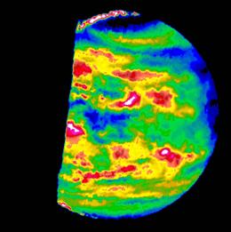
Figure 7.a.7
Picture of the IR radiation of Venus
Question 7.a.4
Why does the radiative equilibrium temperature predicted in our Earth model differ from the actual surface temperature of today’s Earth (~300 K)? What factors have not yet been included in our model, but could be?
Question 7.a.5
In the Earth model, it only took ¼ of a year to reach an equilibrium temperature. This is a very short time compared to the age of the actual Earth. If this time calculation were accurate, what would the implications be for the diversity of life on Earth? Use biologically relevant information to support your answer.
Sources
The image at the top of this
page is from NASA's Solar and
Heliospheric Observatory
http://photojournal.jpl.nasa.gov/jpegMod/PIA00112_modest.jpg
http://wikyonos.seos.uvic.ca/climate-lab/front_page_pics/temperature.lrg.jpeg