Unit 6a. Population Dynamics
 Objective
The goal of this lab is to explore global population growth using STELLA. Historically human population has grown very slowly. However, this pattern has been disrupted within the last two centuries by exponential human population growth rates.
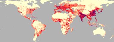
Figure 6.a.1
Global population
World population now stands at more than 6 billion people and is projected to continue growing through this century. Since the world population is estimated to have been 1.6 billion people at the beginning of the 20th century, this means that global population increased by four fold in only 100 years. This unprecedented increase in global population is due to a number of factors that decreased mortality rates worldwide. Factors that increased life expectancy include, better sanitation, increased agriculture, and antibiotic, vaccine, and pesticide use (Environmental Literacy Council, 2005).
The Global human population is expected to continue to rise over the next twenty years or more due to a large number of women reaching child bearing age. Recent estimates predict that the population will continue to increase by ~1.3 percent per year, adding about 78 million people each year (ELC, 2005).
Although the global population growth rate has slowed in recent years, the population is estimated to continue to grow over the next twenty years or more. Most of the increase will occur in nations that have the lowest income levels, depend heavily on natural resources and in areas of rich biological diversity where deforestation for fuel wood and cropland is a serious concern (ELC, 2005).
|
This rapid population growth has been associated with global environmental changes including:
|
Demographic Transitions
To understand this overall pattern of population growth, it is useful to review a basic condition of demographic history, known as the demographic transition: the change of a population from high birth and death rates to low birth and death rates. The demographic transition generally occurs in four stages.
- In the initial stage, both birth and death rates are high, causing only slow and steady population growth.
- In the next stage, death rates begin to decline and birth rates remain high, resulting in faster population growth.
- In stage three, the birth rate begins to decline, and in the final stage, birth rates balance death rates.
- Population
growth stabilizes in this final stage. In some cases, such as
The following two charts illustrate this change.
Figure 6.a.2
Past and present demographic
transition
The Past Demographic Transition
It is important to note that this same transition took place
in every industrialized country in the world (all of Europe and
In developed countries, the decline in death rates was due to three major factors: the trade revolution, the agricultural revolution and the industrial revolution. All of these changes were gradual, and increased the general standard of living for the population, without major medical breakthroughs.
The Present Demographic Transition
Today, the same demographic transition is occurring throughout the world’s less developed countries, though the chart shows some dramatic differences with the past transition.
- First, birth and death rates start at higher levels, for reasons that are not at all clear.
- Second, death rates have declined much more drastically, moving as much in one generation as it had in the past in two centuries.
- Third, the cause of the mortality decline lies in the development of new medical and public health technologies, based on anti-bacterial chemicals and insecticides that reduce disease vectors.
- Rapid mortality declines without concomitant fertility declines means higher rates of population growth are occurring.
The worldwide total fertility rate was estimated to be 5 births per woman when total fertility rates peaked during the period from 1965 to 1970; it is now estimated at 2.7 births.
Additional demographic trends are emerging: the aging of the population. People are living longer and having fewer children. As a result, the average age of the population is increasing, with a larger percentage of the population aged 65 years or older. The aging of populations will mean that larger numbers will require medical and other social services, services that will be provided by fewer numbers of young, productive workers.
Modeling with STELLA
Explore population growth and the past and present demographic transition by developing models of the dynamics characterizing:
- Exponential growth (J-shaped growth)
- Population growth with a carrying capacity (S-shaped growth)
- The past demographic transition that occurred in developed countries
- The present demographic transition that is occurring in developing countries
Exponential growth (J-shaped growth)
Use Figure 6.a.3 to create your first model.
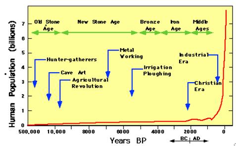
Figure 6.a.3
Human population growth 500,000 years before present to present
Start up STELLA and click on the globe icon so that it changes to a X2 (Chi-square) symbol to begin modeling.
Model the last 2000 years of human
population growth. Global Population will be your stock
![]() .
Use Figure 6.a.3 at 2000 years BP to determine an appropriate initial stock
population.
.
Use Figure 6.a.3 at 2000 years BP to determine an appropriate initial stock
population.
Recall that changes in stocks are modeled in STELLA with the
flow tool: ![]() .
Changes in population are caused by births and deaths.
.
Changes in population are caused by births and deaths.
The final pieces needed for a complete model are birth rate
and death rate. Add this using the converter
tool: ![]() .
.
Use the connector
tool: ![]() to complete the connections in your population model.
to complete the connections in your population model.
Based on the introductory reading, use 2.7 for your average birth rate. Define births with the following equation:
Births=Birth Rate*Population
Add death rate to your model. What would your equation be for deaths? What would be an appropriate death rate? Determine this by changing the death rate to end your model with human population rate at roughly 6 billion people.
Specify an amount of time for the model under Length of Simulation:
From = 0, to = 2000, DT = 10, and Unit of Time = years.
Set up the viewing graph with the graph icon ![]() .
Define your graph with the Population stock.
.
Define your graph with the Population stock.
Add an end value to your model using the rectangle icon. Define it with your population stock. This will give you the ending value of your population at the end of the model run.
Run your model.
Question 6.a.1
What happens when you run your model to 2150? How many people will be living on the planet according to your model?
A More Realistic Model
The model we have created works well, however all populations have limitations to their growth. How can we fix the model to give a more realistic result? We can show this effect in our model by adding a carrying capacity variable and changing the equation for Births.
Add a converter to the model, below and to the right of the flow icon, and name it Carrying Capacity. Connect it to Births.
Change your equation to include the carrying capacity component of your model.
Births = Birth Rate*Population*(1 - (Population/Carrying Capacity))
Question 6.a.2
What do you think is an appropriate carrying capacity for Earth? Why? Add this value to your model and run it. What happens to your population?
Modeling the Past and Present Demographic Transition
Now that you have a grasp on basic human population dynamics, we will explore the past and present demographic transition using STELLA. Open a new STELLA modeling page, copy and paste the model you have created that includes the carrying capacity. You will then alter the model to characterize the past demographic transition. Once the paste demographic transition has been characterized you will copy and paste this model, then alter it to characterize the present demographic transition. Recall that:
- The past demographic transition occurred in developed countries from ~1700 to 2000
- The present demographic transition is occurring in developing countries from 1900 onward
Modeling the Past Demographic Transition
- First change your time specs to 0 to 300, which is the appropriate time based on the past demographic transition. Set your DT=1.
- Click on the Birth rate icon and change the value to the word "Time". Then click on become graphical function. Change the maximum value to 5 and your time from 0 to 300. Then change your graph to match the birth rate in the past demographic transition in Figure 6.a.2 by dragging your mouse on the graph. Hit OK.
- Click on the Death rate icon and again change the value to the word "Time". Click on become graphical function. Change the maximum value to 5 and your time from 0 to 300. Then change your graph to match the death rate in the past demographic transition in Figure 6.a.2 by dragging your mouse on the graph. Hit OK.
- In addition to your global population graph viewer, create a new graph that shows birth and death rates.
- Run your model. Make sure that your birth and death rates make sense. Note that sometimes the scales are different.
Modeling the Present Demographic Transition
- Copy your past demographic transition model, and paste it on a new STELLA workspace. Repeat the steps completed for the past demographic transition for your new model but this time, alter it for the present demographic transition.
- Use 0 to 100 for your time frame.
- Use the appropriate birth and death trends for the present transition as seen in Figure 6.a.2.
Questions
Question 6.a.3
Compare the global population rates at the end of your simulations. What do you see?
Question 6.a.4
Explain the difference between J and S shaped curves. How does carrying capacity of a population influence these relationships?
Question 6.a.5
Does our environment today limit us? What may influence the carrying capacity of our environment (the Earth)?
Question 6.a.6
What adverse effects might the human population experience as we get closer to our carrying capacity? In what forms (biological, social, political) would these adverse effects occur?
Question 6.a.7
What other factors influence population growth? What other converter could be added to your model? How would it affect population dynamics?
Sources
http://www.enviroliteracy.org/subcategory.php/30.html