Unit 3a. Natural Selection and Mutation - The Case of the Peppered Moth
 Objective
The purpose of this lab exercise is to model the effects of natural selection on the appearance and genetic make-up of a natural population (the peppered moth). We will construct a STELLA model for this population that incorporates the basic principles of population genetics.
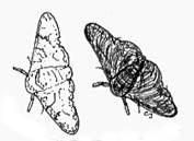
Figure 3.a.1
The peppered moth (Biston betularia)
Before we begin, we will need to define some important genetics terminology:
- Alternative forms of a gene are called alleles
- The genetic constitution of an individual is called its genotype
- The physical expression of a genotype is called the phenotype
- If two alleles are identical, an individual is said to be homozygous for that gene; if two alleles are different, the individual is said to be heterozygous
- A dominant
allele has such a strong phenotypic effect in heterozygous individuals
that it conceals the presence of the weaker (recessive) allele
Introduction
The case of the peppered moth (Biston
betularia)
is a classic example of evolution through directional selection (selection
favoring extreme phenotypes). Prior to the industrial revolution in
The allele (version of the gene) for dark body color is dominant, which means that a moth possessing at least one such allele will have a dark body. (Each individual will have two copies of the gene–one from each of its parents.) To have a light body, the moth has to have both alleles for light body color.
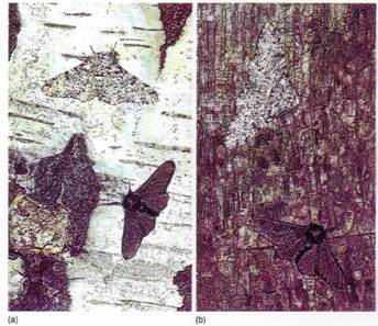
Figure 3.a.2
Dark and light phenotypes of the peppered moth on dark and light barked trees
Dark moths were at a distinct disadvantage, however, due to their increased vulnerability to bird predation. Thus the frequency of the dark allele was very low (about .001%), maintained primarily by spontaneous mutations from light to dark alleles. By 1819, the proportion of dark moths in the population had increased significantly. Researchers found that the light-colored lichens covering the trees were being killed by sulfur dioxide emissions from the new coal burning mills and factories built during the industrial revolution. Without the light background of the trees, the light moths were more visible to vision-oriented predators (birds). They were losing their selective advantage to the dark moths, which, against the trees’ dark bark background, were less visible to birds. In 1848, the dark moths comprised 1% of the population and by 1959 they represented ~90% of the population. So, in 100 years the frequency of dark moths increased by 1000 fold!
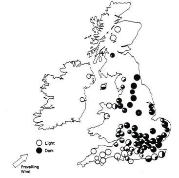
Figure 3.c.3
Composition of various populations
of the peppered moth in the
In this exercise, we will construct a model simulating the
effects of differential predation pressures on a hypothetical peppered moth
population. To do this, we will need to incorporate the genetics of moth body
color into a population dynamics model. We are assuming that body color is the
only trait that confers any significant selective advantages on peppered moths.
Building the Model
Use the diagram below as a guide to help you build the
model. You may want to refer to the Appendix
I. Guide to Basic STELLA Features to help build the model. Keep in
mind that you will have to use ghosts ![]() to
create copies for duplicate variables. However, it is extremely important to make the "Total Moths" converter
in the lower part of the model the original. Make sure the ghost stocks are in the lower part of the model. Then,
all the other ones can be ghosts copied off of it.
to
create copies for duplicate variables. However, it is extremely important to make the "Total Moths" converter
in the lower part of the model the original. Make sure the ghost stocks are in the lower part of the model. Then,
all the other ones can be ghosts copied off of it.
Figure 3.a.4
STELLA model of the peppered moth
As with any system, we must first identify and define the stocks and flows of the system.
Stocks
We have three different genotypes represented in our model:
- AA mothies: homozygous dominant moths that are dark in color
- Aa mothlets: heterozygous moths that are also dark in color
- aa moths: homozygous recessive moths that are light in color
Note: STELLA will not let you repeat variable names. Because STELLA is not case sensitive, it doesn’t distinguish between the names "aa moths" and "Aa moths," so make sure to vary them (i.e. "moths" vs. "mothlets.")
Flows
The flows of our genotypic subpopulations are birth and death. First, take a look at the births:
- birth1 = (repro rate * total moths) * (big A allele^2)
- birth2 = (repro rate * total moths) * (2*big A allele*little a allele)
- birth3 = (repro rate * total moths) * (little a allele^2)
In these flows, the birth rate is calculated by multiplying the reproduction rate of the total population with the frequency of occurrence specific to that genotype.
The allele frequencies are calculated as:
- big A allele = ( (2*AA mothies/total moths) + (Aa mothlets/total moths) ) / 2
- little a allele = ( (2*aa moths/total moths) + (Aa mothlets/total moths) ) / 2
The term for total moths is calculated by using the ghost ![]() to make copies of the 3 stocks and adding them
together:
to make copies of the 3 stocks and adding them
together:
- total moths = AA mothies + Aa mothlets + aa moths
Also define variables that calculate the relative frequencies of dark moths (AA and Aa) and light moths (aa):
- dark freq = (AA mothies + Aa mothlets) / total moths
- light freq = aa moths / total moths
Now look at the death flows for the stocks:
- death1 = AA mothies * (natural mortality + bird predation dark)
- death2 = Aa mothlets * (natural mortality + bird predation dark)
- death3 = aa moths * (natural mortality + bird predation light)
The death flows incorporate a natural mortality rate as well as death resulting from predation by birds. Notice that the bird predation rates are different for dark and light moths. These two different predation rates are defined by:
- bird predation light = pollution * bird pred rate
- bird predation dark = bird pred rate - ( pollution * bird pred rate )
Bird predation rate and pollution are both proportions between 0 and 1. Notice that with high rates of pollution, bird predation light is higher, while bird predation dark is highest when pollution is low.
Below are the constants and rates that we have chosen for this model:
- repro rate = .055
- natural mortality = .045
- bird pred rate = .04
- pollution = 0.0 (for now)
- AA mothies = 250
- Aa mothlets = 500
- aa moths = 250
Set up two graphs for viewing results. The first (graph 1)
should display dark freq and light freq. Set up the second graph
(graph 2) to display numbers of AA mothies, Aa
mothlets, and aa moths. The run specs for
these runs are starting at 0.0 to 200.0 with a DT = 1.0, and the time units set
for years. Next, set up numeric displays ![]() to observe the numeric changes in allele
frequencies (little a
allele and big A allele.)
Don’t forget to select "retain ending value."
to observe the numeric changes in allele
frequencies (little a
allele and big A allele.)
Don’t forget to select "retain ending value."
Investigating the System
Since pollution is the true driver of the change in genotype frequency in the peppered moth population, it is the variable that we are most interested in modifying. Pollution is a proportional term, i.e. if it is zero there is no pollution and when it equals 1, pollution is at a maximum.
Simulate the following three scenarios with your model. For each scenario, save graphs 1 (phenotypic response) and 2 (genotypic response) and copy and paste them into your word document. Make sure to label each graph with the value of the pollution variable (or write it in a caption under the graph).
- First, run the model with no pollution (pollution = 0).
- Next, run the model with maximum pollution (pollution = 1).
- Finally,
run the model with a changing pollution rate, which we can define
graphically (as opposed to a mathematically). Click on and open the pollution converter, and then
select and click on the TIME function
in the Built-ins list.
(First delete the value in the equation box.) Now click on Become Graphical Function to get to
the graphical function. Notice that the X axis is TIME and the Y axis is pollution.
Change the number at the top of the Y-axis to 1.0 to restrict the range of pollution to between 0 and 1. Make sure the X-axis ranges from 0 to 200, representing a time span of 200 years. Next, using your mouse (or typing in the desired output), draw a graph that starts off at 1 (maximum pollution) and drops rapidly to 0 (no pollution) halfway across the graph (i.e. TIME ~100). Run the model under this pollution scenario, copy and paste the graphs that reflect a drop in pollution near year 100.
Now vary the timing of the drop in pollution by shifting the position of the drop on the X-axis. Note how the timing affects the dynamics of the different genotypes.
Questions
Question 3.a.1
Turn in the graphs showing phenotypic (graph 1) and genotypic (graph 2) responses in the moth population for each of the scenarios that you've tested.
Question 3.a.2
In a paragraph, describe the dynamics you observe in each scenario. What happens to the dark moths (AA and Aa genotypes) when pollution is removed from the system (scenario 3)? Why?
Question 3.a.3
What important assumption have we made concerning population growth in this model? Do you think it is reasonable in this case? Why?
Question 3.a.4
What would you expect to happen (in terms of genotypic and phenotypic frequencies) if pollution levels fluctuated widely? Check out your hypothesis by varying the pollution function (add some spikes and dips to make it highly variable).
Sources
Futuyma, Douglas J. 1979. Evolutionary
Biology. Sinauer Associates,
Hartl, Daniel L. 1988. A Primer of
Population Genetics, second edition. Sinuaer Associates,