Unit 1a. Introduction to Systems Dynamic Modeling with STELLA
Objective
Modeling is the process of simplifying a system we wish to better understand. Systems that can be modeled range from the very simple to the extraordinarily complex. The reason we are using dynamic computer models in this text is to gain a working knowledge of, and an insight into the processes of global change. Because of the complexity of these processes, it is often not enough to read about the workings of these phenomena. We must think about the dynamics of a system, extract critical functioning parts, and attempt to build a model that captures its "essence" by making assumptions to account for external variables.
The Modeling Process
Modeling should be approached in a logical and ordered manner. Though following guidelines may seem tedious and unnecessary at times, it greatly increases the chances that your model will (a) work and (b) be a relatively accurate representation of the actual behavior of a real-life system.
At its essence, modeling is a 5 part process:
1. Define the Problem and the Goals of the Model
This is where most people get into trouble. Aside from programming problems, most models give incorrect results because (a) the system under study was not understood well enough or (b) the modeler did not have a clear idea of what the model was actually supposed to show. Make note of any assumptions needed to simplify the model at this stage.
2. Understand the Real Life System
Figure out the crucial components of the system. (These are represented as stocks, flows, converters and connectors in STELLA.) Exclude any components that are unnecessary. Keep the model as simple as possible, as unnecessary complexity will make it difficult to understand and modify later on.
3. Build the Model
Sketch out the connections between model variables. Once you have made all of the relevant connections, use STELLA icons to build the model.
4. Test and Revise the Model
Run the model with different data in order to find out if it works, what its limitations are, and where and when it breaks down.
5. Verify the Model
Though not always possible, try to test your model against real world data.
Although we will not be strictly following every step of this guideline in the development of the models in this text, it is important that you keep them in mind as you develop them now and especially in the future.
Create Your First Model
The instructions listed below will guide you through the construction of your first computer model. This guide, however, should not be used as a "cookbook". You must think about each step and the reasons why they must occur in that particular order. You may want to refer to the Guide to Basic STELLA Features for help.
To illustrate basic modeling principles and introduce you to
STELLA, we help you develop a simple scaled-down model of the dynamics of a
biological population (1. Define the problem and goals of the model). Consider
the problem of population on
First, sketch out what you think the connections between population
growth and natural resources might be on
When STELLA starts up, you will have a blank page ready for a new model. To get into modeling mode, click once on the globe icon on the left hand side of your screen, so that it changes to a X2 (Chi-square) symbol. You are now ready to start modeling.
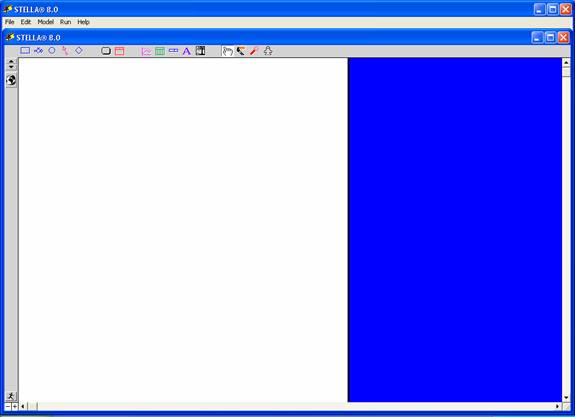
Figure 1.a.1
STELLA modeling interface
The first task in building your model is to establish the
state variable or stock that will
describe the status of the system at each time step.
The symbol for the state variable in STELLA is the stock icon: ![]()
Click on the rectangle icon with your mouse, bring the pointer to the center of your screen and click again. Type in Population for the name of the stock. Inside the population stock icon is a question mark reminding you an initial value is needed. Double-click on the stock icon, and a dialog box will appear asking for a value. Make sure all text is removed prior to typing in the value. Use the keyboard and enter 10 as the initial value, then click on the units button and select people from the business and commerce listing and click OK. You should get into the practice of adding units in your models, which makes results much easier to understand.
We now have the stock that will tell us the status of the system. The next thing that we need is a flow variable that regulates changes in the population.
Changes in stocks are modeled in STELLA with the flow tool: ![]()
Changes in population are caused by births and deaths. Click on the flow icon and bring the pointer to the left of the Population stock. Click and hold, while dragging the arrow to Population so that the box darkens, indicating that the flow has been connected to the stock. Make sure there is only one "cloud" attached to the flow icon. (This can be tricky, so be patient.)
Make sure flows are connected to stocks. Flows must be added to a model after stocks have been laid down. Flows and stocks are connected when the cloud icon disappears at the connection point and the arrow point is on the edge of the stock icon as in Figure 1.a.2.
Figure 1.a.2
Connecting flows to stocks
To add a flow coming out of the stock, make sure that you start the flow inside the stock box and drag it out of the stock while holding down the mouse.
Name the flow
Births. If you make a mistake and
the flow is not connected to the
Population stock, click and drag
the flame of the dynamite icon ![]() on top of the offending flow
icon to blow it up, i.e. to permanently delete it from your model. When the
offending icon changes to a dashed line you can blow it up. Be sure you really
want delete something before using the dynamite
tool.
on top of the offending flow
icon to blow it up, i.e. to permanently delete it from your model. When the
offending icon changes to a dashed line you can blow it up. Be sure you really
want delete something before using the dynamite
tool.
The flow icon should now shows a small "cloud" connected to population by a pipe, which is regulated by a flow valve or gauge you called Births. The cloud represents the source of the material in the stock, in our case people.
The final piece of information needed for a complete model
is the birth rate. We can show this in STELLA using the converter
tool ![]() .
Click and drag the converter icon
to a point below and to the left of the births icon. Label it Birth Rate.
.
Click and drag the converter icon
to a point below and to the left of the births icon. Label it Birth Rate.
It is appropriate to assume that 5 couples had an average of
3 children in a period of 1 year. With 2 adults per couple, this means 3
children divided by 5 couples divided by 2 adults equals 0.3 children per
person per year. Double click on birth rate to open up the dialog box and input
0.3. For units, select "person/time" from units used in this model.
Click OK.
All the pieces are now in place; we just have to connect
them, so that information about one variable can be passed on to other
variables. In STELLA, this is done with the connector tool ![]() .
.
We need Population to be modified by the Birth Rate, so
click on the connector icon,
click on Birth Rate, and then click, hold and drag the connector to Births until the icon darkens, telling you it
connected. Insert another connector from Population to Births, since births are
dependent on the current population.
Double click on Births to open the control box and notice that the variables
you linked with connectors are in the list in the upper left. Use these to
build the relationship that defines reproduction.
Births=Birth Rate*Population
To specify this in STELLA, click on Birth Rate, then the multiplication sign (*), then Population, and click OK. Use the mouse to select these options, DO NOT try to type in the formula, since it a) takes longer and b) increases the chance of a typo (which will prevent your model from working). The model should now look like Figure 1.a.3
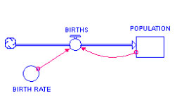
Figure 1.a.3
Population model
It's time to save your model. Your career as a systems modeler will be a lot happier if you remember to save your work often.
To specify an amount of time for the model, say from 1000 AD to 1025 AD, we must first set the time specifications of the simulation (i.e. how long to run, what are the time intervals, etc.) . Under the RUN pull down menu, select Run Specs. In the dialog box, under Length of Simulation, set:
From = 0, To = 25, DT = 1, and Unit of Time = years. Click OK.
Now, to set up the viewing graph, click on the graph
icon ![]() and then on your workspace area. When it is displayed, double click it, and the
dialog box showing the available variables that can be plotted are shown on the
left. If dialog does not appear, click "define graph" on
"Model" menu. Select Population and use the >> button to move it to the Selected box. Click OK to close the dialog box. Resize and move
the window to a good location.
and then on your workspace area. When it is displayed, double click it, and the
dialog box showing the available variables that can be plotted are shown on the
left. If dialog does not appear, click "define graph" on
"Model" menu. Select Population and use the >> button to move it to the Selected box. Click OK to close the dialog box. Resize and move
the window to a good location.
To run the model, select Run under the Run menu. After the data appears on your graph, click on the lock in the bottom left hand corner to keep your graph from changing in subsequent model runs. The graph that appears should look like Figure 1.a.4.
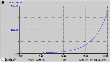
Figure 1.a.4
Graph of population growth
The STELLA modeling system is a user-friendly interface that allows you to build mathematical equations without getting bogged down in the details of programming and complex math. Take a look at the real workings of the model by clicking on the down arrow you see on the extreme left hand side of the screen. The icons you created are translated into difference and differential formulas. Although you will not be expected to interpret the math in these equations, you should be able to see what relationships are being represented.
A More Realistic Model
The model we have just created works well, however, Easter Islanders used the palm trees on the island with no thought about eventual depletion of the resource. How can we fix the model to give a more historically accurate result? (4. Test and revise the model)
We can show this effect in our model by adding a Carrying Capacity variable and changing the equation for Births.
Add a converter to the model, below and to the right of the flow icon, and name it Carrying Capacity. Use a connector to connect it to Births. Double-click on the Carrying Capacity converter to open the dialog box, and input 150. What should the units be? Click OK.
Double click on Births to open the dialog box. Add a term (shown in bold below) to the existing formula using the list of required inputs and the keypad in the dialog box.
Births = Birth Rate*Population*(1 - (Population/Carrying Capacity))
Since the ratio of Population to Carrying Capacity approaches 1 as the Population stock increases, this new term approaches zero. All this really means is that the closer the population gets to the island's carrying capacity, the smaller the increase in births for that time step. The model should now look like Figure 1.a.5.
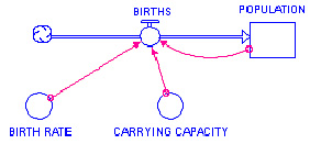
Figure 1.a.5
Population model with carrying capacity
Add a new graph. Run the model with the same time specs. The new graph should look like Figure 1.a.6.
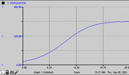
Figure 1.a.6
Population growth with carrying capacity
Judging by the graph, this model seems to be more in line with the way a population might increase in an environment with finite resources.
Summary
In this lab exercise we developed two simple models of population increase using the STELLA modeling tool. Through critical thinking about the system, we identified the stock which we used to monitor the system, the flow which controls changes in the stock and the converter which modifies the flow. The first model represents a population that grows regardless of the limitations of its environment: exponential or J shaped growth. The second model represented a population limited by its environment: logistic or S shaped growth.
Assignment
Since we judged the first model unrealistic, which had the population grow without regard to its environment, we should look at a graph of human population growth throughout history and consider how our entire species has been growing. (5. Verify the model)
Figure 1.a.7
Population growth over time
Look at the shape
of the curve in Figure 1.a.7 and answer questions 1 and 2.
Question 1.a.1
Is the curve shown above more like the curve of the first model or the second model we built? What does this mean for the possible future of the human population?
Question 1.a.2
Do you think current humans are
limited by our environment, just like the people on
Question 1.a.3
By the 19th century there were
fewer than 100 people living on