Unit 10a.2. Alteration of the Global Carbon Cycle
 Objective
Precise records of past and present atmospheric CO2
concentrations are critical to studies attempting to model and understand the
global carbon cycle and possible CO2 -induced climate change.
Researchers have attempted to determine past levels of atmospheric CO2 concentrations
by a variety of techniques, including direct measurements of trapped air in polar
ice cores; and indirect determinations from carbon isotopes in tree rings,
analysis of spectroscopic data, and measurements of carbon and oxygen isotopic
changes in deep-ocean sediments. The modern period of precise atmospheric CO2
measurements began during the International Geophysical Year (1958) with Keeling's (Scripps Institution of Oceanography) pioneering
determinations at
Figure 10.a.2.1
Carbon cycle
In this lab exercise we will do the following:
- Examine the Mauna Loa CO2 data.
- Build a STELLA model of the global carbon cycle in order to understand natural and anthropogenic processes in this cycle.
- Develop future carbon cycle scenarios and analyze them to determine possible effects on global climate change.
Part 1: Mauna Loa Atmospheric CO2
Concentrations
Examine the
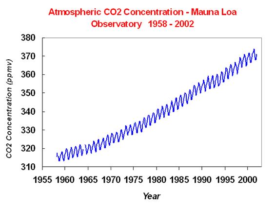
Figure 10.a.2.2
CO2 concentration from 1958 to 2002
Part 2: Modeling Changes in Atmospheric Carbon Using STELLA
Create a working STELLA model of the global carbon cycle. First, determine the number of stocks in the carbon cycle and place them on your STELLA workspace. Next, make the relevant connections between the stocks using the flow symbols, and add the appropriate converters. (To bend flow arrows, hit the Shift key where you want to insert a "kink" in the flow.) When the model structure has been fully laid out, assign the values given below. (One gigaton = 10 15g.). Switch to modeling mode by turning the Globe into the X2 icon.
Change the Run Specs so that the simulation runs from 1958
to 2002 (corresponding approximately with the
You are now ready to explore the effect of fossil fuels on
CO2. Experiment with different values for fossil fuel combustion to
get a graph of Atmospheric CO2 (ppm) that
is similar to the graph we created for the ![]() for this variable.
for this variable.
Stock #1: Atmospheric Carbon
Initial Value (1958) = 720 {gigatons}
Inflows
- Ocean Release = 105 {gigatons/yr.}
- Respiration = 60 {gigatons/yr.}
- Deforestation = 1.8 {gigatons/yr.}
- Exhalation = 60 {gigatons/yr.}
- Fossil Fuel Combustion = ?
Outflows
- Ocean Uptake = 106.6 {gigatons/yr.}
- Photosynthesis = 80 + NH Photosynthesis {gigatons/yr.}
- Unknown
Sink = 2.2 {gigatons/yr.}
Stock #2: Land Plants
Initial Value (1958) = 560 {gigatons}
Inflows
- Photosynthesis (see above)
Outflows
- Detritus = 60.4 {gigatons/yr.}
- Deforestation (see above)
- Respiration
(see above)
Stock #3: Ocean Carbon
Initial Value (1958) = 38000 {gigatons}
Inflows
- Runoff = 0.4 {gigatons/yr.}
- Ocean Uptake (see above)
Outflows
- Sediments = 0.1 {gigatons/yr.}
- Ocean
Release (see above)
Stock #4: Soils
Initial Value (1958) = 1500 {gigatons}
Inflows
- Detritus (see above)
Outflows
- Exhalation (see above)
- Runoff (see above)
Converters
- Atmospheric CO2 ppm = 310 * (Atmospheric Carbon / 720)
- NH (Northern Hemisphere) Photosynthesis = PI*40*MAX(0,SIN(2*PI*(Season-0.25))) (Use the built-ins to input this)
- Season
= TIME-INT(TIME) (Use the built-ins to input this)
Questions
Question 10.a.2.1
Run the model forward in time to determine when the estimated CO2 reaches 600 ppm. (You will need to change the Run Specs to do this.) Give a brief qualitative explanation of how you think this increased CO2 concentration will affect global climate. Be sure to cite relevant scientific information to support your answer and include the date determined above. Include your STELLA graph of Atmospheric CO2 (ppm) and note the value you used for fossil fuel combustion.
Question 10.a.2.2
Explain the annual seasonal
variation that you built into your model and that you see in the
Question 10.a.2.3
Look at the processes in the global carbon cycle, and identify the anthropogenic (human-made) factors. By altering one or more of these, develop a possible future scenario of the carbon cycle and model it in STELLA. Hand in your new (relabeled) graph of Atmospheric CO2 (ppm). Describe the factors you changed and how these changes affected global climate.
Question 10.a.2.4
Given the mass balance calculations that have been done with known concentrations of atmospheric carbon, we need a "sink" to balance the global C budget. In other words, we are "missing" over 2 billion tons of C each year; this shows how incomplete our understanding of the global carbon cycle is at present. What are some of the scientific speculations about where this missing sink could be located? Name at least two.
Sources
http://www.pewclimate.org/global-warming-in-depth/all_reports/land_use_and_climate_change/index.cfm
Classroom of the Future, Earth
on Fire Modules: Carbon Cycle.
http://www.cotf.edu/ete/modules/carbon/efcarbon.html
http://www.ucar.edu/learn/images/carboncy.gif